Matrix Lie Group
In this chapter, we will talk about the matrix Lie Group and its Lie Algebra. Matrix Lie Group and Algebra provides rigious math models for rigid body transformation and rotation matrix. Understanding Matrix Lie Group and Lie Algebra is not only important for knowing rigid body trasnformation further, but also the keys to the optimization problems over rigid body transformation, such as reprojection error optimization in visual SLAM. Before diving into the technical details, it is recommended to watch this tutorial video about Lie Group and Lie Algebra.
Group Perspective
Formally, rotation matrix $\mathbf{R}$ is a $n$ dimensional Special Orthogonal (SO) Group, which is,
$$
\begin{align}
\mathrm{SO}(n) =
\left\{ \mathbf{R} \in \mathbb{\mathbf{R}}^{n \times n} \vert \mathbf{R}\mathbf{R}^{\top} = \mathbf{I}, \det(\mathbf{R}) = 1 \right\}
\end{align}
$$
Obviously, the 3D rotation matrix we talked about is $\mathrm{SO}(3)$ group.
The previously mentioned 3D rigid body motion is also a Lie Group, which is called Special Euclidean (SE) Group, $\mathrm{SE}(3)$. It has $\mathrm{SO}(3)$ and $\mathbb{R}^3$ as its subgroups:
$$
\begin{align}
\mathrm{SE}(3) = \left\{ \mathbf{T} = \begin{bmatrix} \mathbf{R} & \mathbf{t} \\ \mathbf{0} & 1 \end{bmatrix} \in \mathbb{\mathbf{R}}^{4 \times 4}: \mathbf{R} \in \mathrm{SO}(3), \, \mathbf{t} \in \mathbb{R}^3 \right\}
\end{align}
$$
In the languange of abstract algebra, a Group is an algebraic structure consisting of a set, denoted as $S$, and an operation, denoted as $\cdot$. $G = (S, \cdot)$ is a group if the operation $\cdot$ satisfies the following conditions:
- Closure:
\( \forall a_1, a_2 \in S, \ a_1 \cdot a_2 \in S. \)
- Associativity:
\( \forall a_1, a_2, a_3 \in S, \ (a_1 \cdot a_2) \cdot a_3 = a_1 \cdot (a_2 \cdot a_3). \)
- Identity element:
\( \exists a_0 \in S \) such that \( \forall a \in S, \ a_0 \cdot a = a \cdot a_0 = a. \)
- Inverse element:
\( \forall a \in S, \ \exists a^{-1} \in S \) such that \( a \cdot a^{-1} = a^{-1} \cdot a = a_0. \)
A Lie Group is a group that is also a differentiable manifold. A manifold is a topological space that locally resembles Euclidean space. Manifold is anywhere, the earth surface is a manifold, the spacetime we live in is a manifold. We first talk about why rotation and rigid body transformation is roups, then we talk about why they are also manifolds. Lie Group is named after the Norwegian mathematician Sophus Lie (1842-1899).
Let's first prove the rotation matrix and rigid body transformation are groups. The proof is actually rather straightforward.
1. Closure
It's obvious to find a operation (actually the only operation) that satisfies the closure property for $\mathrm{SO}(3)$ and $\mathrm{SE}(3)$, which is matrix multiplication.
Given $\mathbf{R}_1, \mathbf{R}_2 \in \mathrm{SO}(3)$, the group operation is:
$$
\begin{align}
\mathbf{R}_1 \mathbf{R}_2 \in \mathrm{SO}(3)
\end{align}
$$
Given $\mathbf{T}_1, \mathbf{T}_2 \in \mathrm{SE}(3)$, the group operation is:
$$
\begin{align}
\mathbf{T}_1 \, \mathbf{T}_2 = \begin{bmatrix} \mathbf{R}_1 \mathbf{R}_2 & \mathbf{R}_1 \mathbf{t}_2 + \mathbf{t}_1 \\ \mathbf{0} & 1 \end{bmatrix} \in \mathrm{SE}(3)
\end{align}
$$
It's also obvious that addition/subtraction is not a valid operation for $\mathrm{SO}(3)$ and $\mathrm{SE}(3)$, since
$$
\begin{align}
\mathbf{R}_1 + \mathbf{R}_2 \notin \mathrm{SO}(3); \quad \mathbf{T}_1 + \mathbf{T}_2 \notin \mathrm{SE}(3)
\end{align}
$$
2. Associativity
Associativity is also obvious for $\mathrm{SO}(3)$ and $\mathrm{SE}(3)$, since matrix multiplication is simply associative.
3. Identity element
The identity element for $\mathrm{SO}(3)$ and $\mathrm{SE}(3)$ is a $3 \times 3$ and $4 \times 4$ identity matrix, respectively.
$$
\begin{align}
\mathbf{I}_3 \in \mathrm{SO}(3); \quad \mathbf{I}_4 \in \mathrm{SE}(3)
\end{align}
$$
4. Inverse element
Inverse of a rotation matrix is its transpose:
$$
\begin{align}
\mathbf{R}^{-1} = \mathbf{R}^{\top}
\end{align}
$$
And the inverse of a rigid body transformation is:
$$
\begin{align}
\mathbf{T}^{-1} =
\begin{bmatrix}
\mathbf{R}^{\top} & -\mathbf{R}^{\top}\mathbf{t} \\
\mathbf{0}^{\top} & 1
\end{bmatrix}
\end{align}
$$
Manifold Perspective
Next we talk about the manifold perspective of the rotation matrix and rigid body transformation. Since they are manifolds, they can be locally approximated by a tangent space, which is a Euclidean space. The following figure illustrates manifold and its local approximation of tangent space.
Lie Algebra, Retract and Exponential Map
To better understand Lie Group/Manifold and Lie Algebra, we need to bring a little taste of differential geometry here.
Lie Algebra of $\mathrm{SO}(3)$
We first start the derivation of Lie Algebra of $\mathrm{SO}(3)$. Think of a camera moving in a 3D space, the rotation matrix $\mathbf{R}(t)$ changes continuously over time, thus defined as a function over time $t$. It should satisfy:
$$
\begin{align}
\mathbf{R}(t)\mathbf{R}(t)^\mathrm{T} = \mathbf{I}
\end{align}
$$
Taking the derivative over time $t$ on both sides of the equation yields:
$$
\begin{align}
\dot{\mathbf{R}}(t)\mathbf{R}(t)^\mathrm{T} + \mathbf{R}(t)\dot{\mathbf{R}}(t)^\mathrm{T} = \mathbf{0}
\end{align}
$$
hence,
$$
\begin{align}
\dot{\mathbf{R}}(t)\mathbf{R}(t)^\mathrm{T} = -\left(\dot{\mathbf{R}}(t)\mathbf{R}(t)^\mathrm{T}\right)^\mathrm{T}
\end{align}
$$
Thus matrix $\dot{\mathbf{R}}(t)\mathbf{R}(t)^\mathrm{T}$ is a skew-symmetric matrix, which means there exists a 3D vector $\boldsymbol{\omega}(t) \in \mathbb{R}^3$ corresponding to the skew-symmetric matrix via the hat operator. And physically, $\boldsymbol{\omega} \in \mathbb{R}^3$ is the angular velocity:
$$
\begin{align}
\label{eq:phi_hat}
\boldsymbol{\omega}(t)^\wedge = \dot{\mathbf{R}}(t)\mathbf{R}(t)^\mathrm{T}
\end{align}
$$
In specific, the hat operator for $\boldsymbol{\omega}$ is defined as:
$$
\begin{align}
\boldsymbol{\omega}^\wedge = [\boldsymbol{\omega}]_\times =
\begin{bmatrix}
0 & -\omega_3 & \omega_2 \\
\omega_3 & 0 & -\omega_1 \\
-\omega_2 & \omega_1 & 0
\end{bmatrix}
\end{align}
$$
This is literally the definition of the cross product.
\begin{equation}
\mathbf{a} \times \mathbf{b} =
\begin{bmatrix}
a_2 b_3 - a_3 b_2 \\
a_3 b_1 - a_1 b_3 \\
a_1 b_2 - a_2 b_1
\end{bmatrix}
=
\begin{bmatrix}
0 & -a_3 & a_2 \\
a_3 & 0 & -a_1 \\
-a_2 & a_1 & 0
\end{bmatrix}
\mathbf{b}
\triangleq {\mathbf{a}}^\wedge \mathbf{b}.
\end{equation}
If we simply manipulate the equation \eqref{eq:phi_hat} by right-multiplying both sides by $\mathbf{R}(t)$, and using the property that $\mathbf{R}(t)$ is an orthogonal matrix, we get the derivative of the rotation matrix over $t$ is simply:
$$
\begin{align}
\label{eq:phi_hat_derivative}
\dot{\mathbf{R}}(t) = \boldsymbol{\omega}(t)^\wedge \mathbf{R}(t)
\end{align}
$$
When $\mathbf{R(t)} = \mathbf{I}$, the derivative of the rotation matrix over $t$ is simply:
$$
\begin{align}
\dot{\mathbf{R}}(t) = \boldsymbol{\omega}(t)^\wedge; \quad \text{or simply} \quad \dot{\mathbf{R}} = \boldsymbol{\omega}^\wedge;
\end{align}
$$
And at this point, we can see that the tangent space, which is reflecting the derivative of the rotation matrix over $t$ at the identity, is a 3-dimensional real vector space, coinciding with the space of $3 \times 3$ skew-symmetric matrices. This tangent space is denoted as $\mathfrak{so}(3)$, defined as the Lie algebra of $\mathrm{SO}(3)$.
\begin{equation}
\mathfrak{so}(3) = \left\{ \boldsymbol{\omega} \in \mathbb{R}^3 \quad \text{or} \quad \boldsymbol{\omega}^\wedge \in \mathbb{R}^{3 \times 3} \right\}
\end{equation}
We will also give the defination of Lie bracket, which is used to preserve the closure of Lie Algebra. Hence, after the Lie bracket operation, the result is still a Lie Algebra. The Lie bracket of $\mathfrak{so}(3)$ is defined as:
$$
\begin{align}
[\boldsymbol{\omega}_1, \boldsymbol{\omega}_2]
= \left( \boldsymbol{\omega}_1^{\wedge} \boldsymbol{\omega}_2^{\wedge} - \boldsymbol{\omega}_2^{\wedge} \boldsymbol{\omega}_1^{\wedge} \right)^{\vee}
\end{align}
$$
We mapping between Lie Algebra $\mathfrak{so}(3)$ and vector space $\mathbb{R}^3$is through the linear operators hat and vee,
$$
\begin{align}
\mathbb{R}^3 \rightarrow \mathfrak{so}(3); \quad \boldsymbol{\omega} \mapsto \boldsymbol{\omega}^\wedge = [\boldsymbol{\omega}]_\times
\end{align}
$$
$$
\begin{align}
\mathfrak{so}(3) \rightarrow \mathbb{R}^3; \quad [\boldsymbol{\omega}]_\times \mapsto [\boldsymbol{\omega}]_\times^\vee = \boldsymbol{\omega}
\end{align}
$$
The solution to the differential equation \eqref{eq:phi_hat_derivative} is:
$$
\begin{align}
\mathbf{R}(t) = \exp\left(\boldsymbol{\omega}(t_0)^\wedge t\right)
\end{align}
$$
We further assign the rotation vector as $\boldsymbol{\phi} = \boldsymbol{\omega} t$. For notational simplicity, we omit the subscript 0 and define the mapping from a small rotation vector $\boldsymbol{\phi} \in \mathbb{R}^3$ to the rotation matrix as:
$$
\begin{align}
\label{eq:exp_map}
\mathbf{R}(t) = \exp\left(\boldsymbol{\phi}^\wedge\right)
\end{align}
$$
Note that $\boldsymbol{\phi} \in \mathfrak{so}(3)$ is also the Lie Algebra of $\mathrm{SO}(3)$.
This mapping is denoted as Exponential Map, which is a mapping from the Lie Algebra ($\mathfrak{so}(3)$) to the Lie Group ($\mathrm{SO}(3)$). This process is also called Retraction.
Equation \eqref{eq:exp_map} can be rewritten using the Taylor series expansion. First recall the Taylor series expansion of the exponential function for
$$
\begin{align}
\exp(\mathbf{A}) = \sum_{n=0}^{\infty} \frac{\mathbf{A}^n}{n!}.
\end{align}
$$
Then we can rewrite the exponential function for $\boldsymbol{\phi}^\wedge$ as, and here we separate the vector normal and the magnitude of $\boldsymbol{\phi}$ as $\boldsymbol{\phi} = \mathbf{n} \phi$.
\begin{equation}
\begin{aligned}
\mathbf{R} &= \exp(\boldsymbol{\phi}^\wedge) = \exp([\boldsymbol{\phi}]_\times) = \sum_{k=0}^\infty \frac{(\phi [\mathbf{n}]_\times)^k}{k!} = \sum_{k=0}^\infty \frac{\phi^k}{k!} ([\mathbf{n}]_\times)^k \\
&= \mathbf{I} + \phi [\mathbf{n}]_\times + \frac{1}{2!}\phi^2 [\mathbf{n}]_\times^2 + \frac{1}{3!}\phi^3 [\mathbf{n}]_\times^3 + \frac{1}{4!}\phi^4 [\mathbf{n}]_\times^4 + \cdots \\
\end{aligned}
\end{equation}
We compute a few powers of $[\mathbf{n}]_\times$ to find some patterns:
$$
\begin{equation}
[\mathbf{n}]_\times^0 = \mathbf{I}, \quad
[\mathbf{n}]_\times^1 = [\mathbf{n}]_\times, \quad
[\mathbf{n}]_\times^2 = \mathbf{n}\mathbf{n}^\top - \mathbf{I}, \quad
[\mathbf{n}]_\times^3 = -[\mathbf{n}]_\times, \quad
[\mathbf{n}]_\times^4 = -[\mathbf{n}]_\times^2, \quad \cdots
\end{equation}
$$
Then we realize that all powers can be expressed as multiples of $\mathbf{I}$, $[\mathbf{n}]_\times$, or $[\mathbf{n}]_\times^2$.
Thus, we can rewrite the series as:
\begin{equation}
\begin{aligned}
\mathbf{R} &= \mathbf{I} + \phi [\mathbf{n}]_\times + \frac{1}{2!}\phi^2 ([\mathbf{n}]_\times^2) - \frac{1}{3!}\phi^3 [\mathbf{n}]_\times - \frac{1}{4!}\phi^4 ([\mathbf{n}]_\times^2) + \cdots \\
&= \mathbf{I}
+ [\mathbf{n}]_{\times} \left( \phi - \frac{1}{3!} \phi^3 + \frac{1}{5!} \phi^5 \cdots \right)
+[\mathbf{n}]_{\times}^2 \left( \frac{1}{2!} \phi^2 - \frac{1}{4!} \phi^4 + \frac{1}{6!} \phi^6 \cdots \right) \\
&= \mathbf{I} + [\mathbf{n}]_{\times} \sin \phi + [\mathbf{n}]_{\times}^2 (1 - \cos \phi)
\end{aligned}
\end{equation}
This equation is called Rodrigues' rotation formula , named after the French mathematician Olinde Rodrigues (1795-1851).
The first-order approximation of the Exponential Map is:
$$
\begin{align}
\exp(\boldsymbol{\phi}^\wedge) \approx \mathbf{I} + \boldsymbol{\phi}^\wedge
\end{align}
$$
Lie Algebra of $\mathrm{SE}(3)$
Similarly, we derive the Lie Algebra of $\mathrm{SE}(3)$, denoted as $\mathfrak{se}(3)$. $\mathfrak{se}(3)$ is a 6-dimensional real vector space $\boldsymbol{\xi}^\wedge$, coinciding with the space of $4 \times 4$ matrices. Note that $\boldsymbol{\xi}^\wedge$ is no longer a skew-symmetric matrix.
\begin{equation}
\mathfrak{se}(3) = \left\{
\boldsymbol{\xi} =
\begin{bmatrix}
\boldsymbol{\rho} \\
\boldsymbol{\phi}
\end{bmatrix}
\in \mathbb{R}^6, \ \boldsymbol{\rho} \in \mathbb{R}^3, \ \boldsymbol{\phi} \in \mathfrak{so}(3), \
\boldsymbol{\xi}^\wedge =
\begin{bmatrix}
\boldsymbol{\phi}^\wedge & \boldsymbol{\rho} \\
\mathbf{0}^{\top} & 0
\end{bmatrix}
\in \mathbb{R}^{4 \times 4}
\right\}
\end{equation}
There the vector $\boldsymbol{\rho}$ physically represents the a small translation.
And the Lie bracket of $\mathfrak{se}(3)$ is defined as:
$$
\begin{align}
[\boldsymbol{\xi}_1, \boldsymbol{\xi}_2] = (\boldsymbol{\xi}_1^\wedge \boldsymbol{\xi}_2^\wedge - \boldsymbol{\xi}_2^\wedge \boldsymbol{\xi}_1^\wedge) ^\vee
\end{align}
$$
The exponential map of $\mathfrak{se}(3)$ is:
\begin{equation}
\begin{aligned}
\exp(\boldsymbol{\xi}^\wedge) &= \sum_{k=0}^{\infty} \frac{1}{k!} ({\boldsymbol{\xi}^\wedge})^k \\
&= \sum_{k=0}^{\infty} \frac{1}{k!}
\begin{bmatrix}
\boldsymbol{\phi} \\
\boldsymbol{\rho}
\end{bmatrix}^\wedge \\
&= \sum_{k=0}^{\infty} \frac{1}{k!}
\begin{bmatrix}
{\boldsymbol{\phi}^\wedge} & \boldsymbol{\rho} \\
\mathbf{0}^T & 0
\end{bmatrix}^k \\
&= \sum_{k=0}^{\infty} \frac{1}{k!}
\begin{bmatrix}
(\boldsymbol{\phi}^\wedge)^k & (\boldsymbol{\phi}^\wedge)^{k-1} \boldsymbol{\rho} \\
\mathbf{0}^T & 0
\end{bmatrix} \\
&=
\begin{bmatrix}
\sum\limits_{k=0}^\infty \frac{1}{k!} (\boldsymbol{\phi}^\wedge)^k & \sum\limits_{k=0}^\infty \frac{1}{(k+1)!} (\boldsymbol{\phi}^\wedge)^k \boldsymbol{\rho} \\
\mathbf{0}^{\top} & 1
\end{bmatrix} \\
&= \begin{bmatrix}
\exp(\boldsymbol{\phi}^\wedge) & \mathbf{J}(\boldsymbol{\phi}) \boldsymbol{\rho} \\
\mathbf{0}^{\top} & 1
\end{bmatrix} \\
&=
\begin{bmatrix}
\mathbf{R} & \mathbf{t} \\
\mathbf{0}^{\top} & 1
\end{bmatrix}
= \mathbf{T}
\end{aligned}
\end{equation}
We see that after passing the exponential map, the translation part is multiplied by a linear Jacobian matrix $\mathbf{J}(\boldsymbol{\phi})$, hence
\begin{equation}
\mathbf{t} = \mathbf{J}(\boldsymbol{\phi}) \boldsymbol{\rho}
\end{equation}
where $\mathbf{J}(\boldsymbol{\phi})$ is the left Jacobian of $\boldsymbol{\phi}$:
\begin{equation}
\label{eq:jacobian_so3}
\mathbf{J}(\boldsymbol{\phi}) = \sum\limits_{k=0}^\infty \frac{1}{(k+1)!} (\boldsymbol{\phi}^\wedge)^k
\end{equation}
We will visit more about Jacobian matrix $\mathbf{J}(\boldsymbol{\phi})$ applied in derivatives of $\mathrm{SO}(3)$ and $\mathrm{SE}(3)$ in the next section.
Local Operations via Logarithm Map
We've walked thought the mapping from Lie Algebra to Lie Group. Next we talk about the inverse process, which is called Local operation via the Logarithm Map, which literally means take the local linear approximation of the Lie Group.
Again, starts from $\mathrm{SO}(3)$, the logarithm of a rotation matrix $\mathbf{R} \in \mathrm{SO}(3)$ can be derived from Rodrigues' formula:
\begin{equation}
\mathbf{R} = \exp(\phi [\mathbf{n}_\times]) = \mathbf{I} + \sin\phi\, [\mathbf{n}_\times] + (1 - \cos\phi)\, ([\mathbf{n}_\times])^2
\end{equation}
We take the trace operator on both side. and find the angle $\phi$ from $\mathbf{R}$:
\begin{equation}
\begin{aligned}
\mathrm{tr}(\mathbf{R})
&= \mathrm{tr}(\mathbf{I}) + \sin(\phi) \mathrm{tr}([\mathbf{n}_\times]) + (1 - \cos(\phi)) \mathrm{tr}([\mathbf{n}_\times]^2) \\
&= 3 + \sin(\phi) \cdot 0 + (1 - \cos(\phi)) (-2) \\
&= 1 + 2\cos(\phi)
\end{aligned}
\end{equation}
Hence $\phi$ is solved as:
\begin{equation}
\phi = \cos^{-1}\left(\frac{\mathrm{tr}(\mathbf{R}) - 1}{2}\right)
\end{equation}
Then we can find the axis $\mathbf{n}$ from $\mathbf{R}$:
Apply the Rodrigues' formula to $\mathbf{R}^{-1} = \mathbf{R}^\top$, we get:
\begin{equation}
\mathbf{R}^{\top} = \exp(-\phi [\mathbf{n}_\times]) = \mathbf{I} + \sin (-\phi) [\mathbf{n}]_{\times} + (1 - \cos (-\phi)) [\mathbf{n}]_{\times}^2
\end{equation}
Do a simple substitution, we get:
\begin{equation}
\mathbf{R} - \mathbf{R}^\top = 2\sin\phi\, [\mathbf{n}_\times]
\end{equation}
then the normal vector $\mathbf{n}$ is solved as:
\begin{equation}
[\mathbf{n}_\times] = \frac{\mathbf{R} - \mathbf{R}^\top}{2\sin\phi}
\end{equation}
Finally, the logarithm of rotation matrix $\mathbf{R}$ is:
\begin{equation}
\ln(\mathbf{R}) = \phi [\mathbf{n}_\times] = \frac{\phi (\mathbf{R} - \mathbf{R}^\top)}{2\sin\phi}
\end{equation}
The logarithm map can also be derived from the Taylor expansion of the Logarithm function:
\begin{equation}
\ln(\mathbf{R}) = \sum\limits_{k=1}^\infty \frac{(-1)^{k+1}}{k} (\mathbf{R} - \mathbf{I})^k
\end{equation}
And here note that $\mathbf{R} \neq \mathbf{I}$ in general.
In summary, the mapping between Lie Algebra and Lie Group is through the exponential map and logarithm map:
$$
\begin{align}
\mathrm{Exp}: \mathbb{R}^3 \rightarrow \mathrm{SO}(3), \quad \boldsymbol{\phi} \mapsto \exp(\boldsymbol{\phi}^\wedge)
\end{align}
$$
$$
\begin{align}
\mathrm{Log}: \mathrm{SO}(3) \rightarrow \mathbb{R}^3, \quad \mathbf{R} \mapsto \ln(\mathbf{R})^\vee
\end{align}
$$
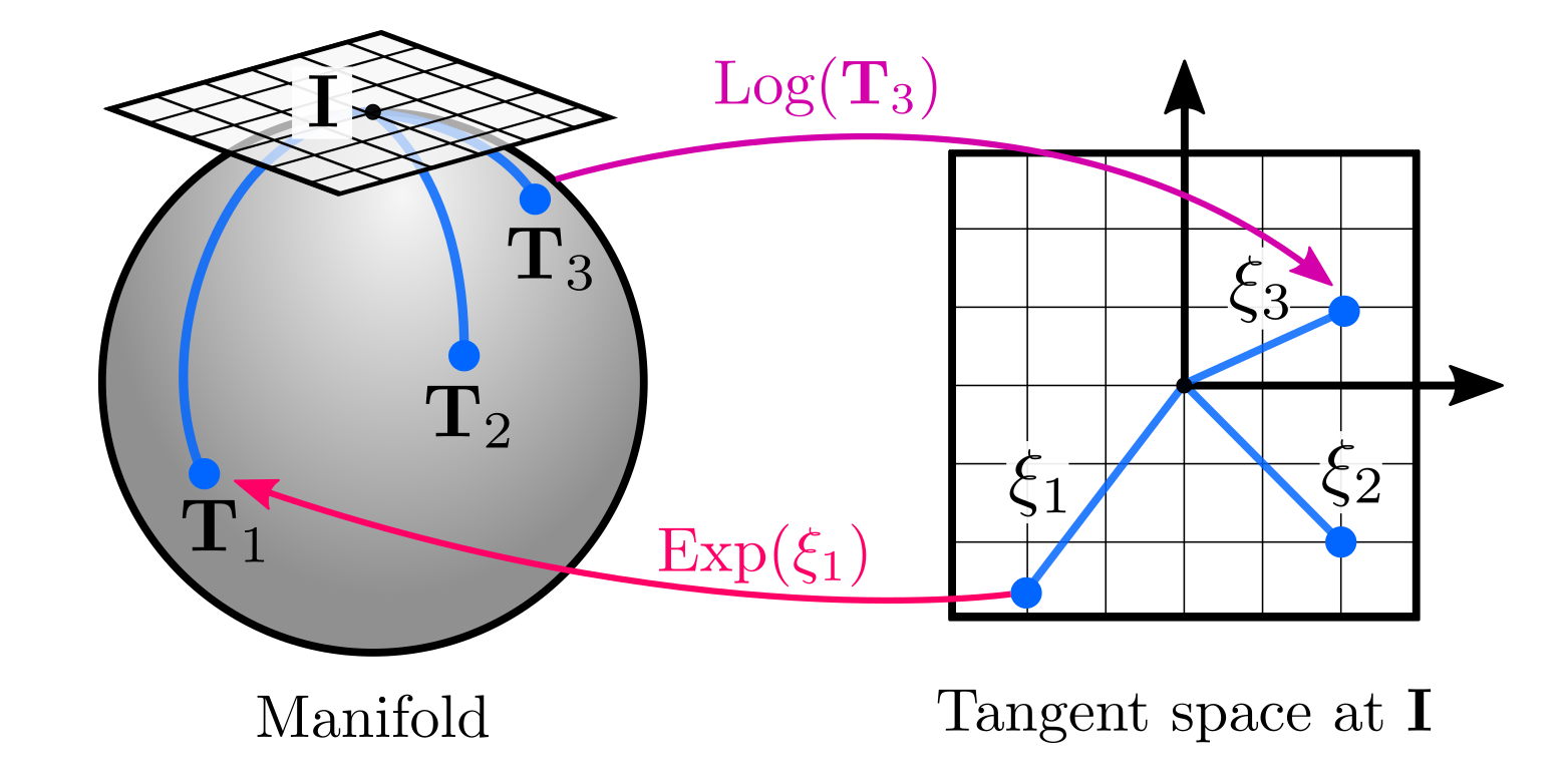
The following figure is an excellent illustration of the Exponential and Logarithm maps. Note this figure also illutrates the defination of Lie Algebra as the tangent space of the Lie Manifold is at the identity element of the Lie Manifold.
BCH Formula
Before we move to the Jacobian of Lie Group/Algebra, let's talk about the BCH formula. BCH formula is a key tool to get the results of two elements in Lie Group, which is then used to derive the Jacobian of Lie Algebra.
Let's start with regular matrices $\mathbf{X}, \mathbf{Y} \in \mathbb{R}^{n \times n}$, we have
\begin{equation}
\exp(\mathbf{X}) \exp(\mathbf{Y}) = \exp(\mathbf{X} + \mathbf{Y})
\end{equation}
This does not hold for Lie Algebra, though. To connect two Lie algebra elements $\mathbf{A}, \mathbf{B} \in \mathfrak{so}(3)$, we can use the Baker-Campbell-Hausdorff (BCH) formula :
\begin{equation}
\ln\left( \exp(\mathbf{A}) \exp(\mathbf{B}) \right)
= \mathbf{A} + \mathbf{B}
+ \frac{1}{2} [\mathbf{A}, \mathbf{B}]
+ \frac{1}{12} [\mathbf{A}, [\mathbf{A}, \mathbf{B}]]
- \frac{1}{12} [\mathbf{B}, [\mathbf{A}, \mathbf{B}]]
+ \cdots
\end{equation}
Where operation $[, ]$ denotes the Lie bracet.
Jacobian of Lie Group and Algebra
BCH Formula Revisited
Let's just pause for a moment and think about why we are doing all these previous derivations, actually they mainly serve the derivation of the Jacobian of Lie Group and Algebra, which is the key to the optimization problem over Rigid body transformation SE(3) and SO(3).
Now let's apply BCH formula to build the how small pertabulations on $\mathfrak{so}(3)$ and $\mathfrak{se}(3)$ applied in exponential maps.
First, with small perturbation $\delta \boldsymbol{\phi} \in \mathfrak{so}(3)$, and apply first order approximation of BCH formula, we have:
\begin{equation}
\exp\left( \delta \boldsymbol{\phi}^\wedge \right) \exp\left( \boldsymbol{\phi}^\wedge \right)
\approx \exp \left( \left( \boldsymbol{\phi} + \mathbf{J}_l^{-1}(\boldsymbol{\phi}) \delta \boldsymbol{\phi} \right)^\wedge \right)
\end{equation}
\begin{equation}
\exp\left( \boldsymbol{\phi}^\wedge \right) \exp\left( \delta \boldsymbol{\phi}^\wedge \right)
\approx \exp \left( \left( \boldsymbol{\phi} + \mathbf{J}_r^{-1}(\boldsymbol{\phi}) \delta \boldsymbol{\phi} \right)^\wedge \right)
\end{equation}
where $\mathbf{J}_l(\boldsymbol{\phi})$ is defined as the left Jacobian of $\boldsymbol{\phi}$, and $\mathbf{J}_r(\boldsymbol{\phi})$ is defined as the right Jacobian of $\boldsymbol{\phi}$ (which is the inverse of the left Jacobian).
\begin{equation}
\mathbf{J}_r(\boldsymbol{\phi}) = \mathbf{J}_l(-\boldsymbol{\phi}).
\end{equation}
These two Jacobians maps the small pertabulation on $\delta \boldsymbol{\phi} \in \mathfrak{so}(3)$ to the small pertabulation on $\mathrm{SO}(3)$, near $\boldsymbol{\phi}$.
We shall next how the small perturbations directly applied on $\mathfrak{so}(3)$ before exponential map, hence adding the small perturbation on $\mathfrak{so}(3)$ directly.
\begin{equation}
\exp \left( (\boldsymbol{\phi} + \delta \boldsymbol{\phi})^\wedge \right)
\approx \exp \left( (\mathbf{J}_l (\boldsymbol{\phi}) \delta \boldsymbol{\phi})^\wedge \right)
\exp \left( \boldsymbol{\phi}^\wedge \right)
= \exp \left( \boldsymbol{\phi}^\wedge \right)
\exp \left( (\mathbf{J}_r (\boldsymbol{\phi}) \delta\boldsymbol{\phi})^\wedge \right)
\end{equation}
Similarly, for small perturbation $\delta \boldsymbol{\xi} \in \mathfrak{se}(3)$, we have:
\begin{equation}
\exp \left( \delta \boldsymbol{\xi}^\wedge \right) \exp \left( \boldsymbol{\xi}^\wedge \right)
\approx \exp \left( \left( \mathcal{J}_l^{-1}(\boldsymbol{\xi}) \delta \boldsymbol{\xi} + \boldsymbol{\xi} \right)^\wedge \right)
\end{equation}
\begin{equation}
\exp \left( \boldsymbol{\xi}^\wedge \right) \exp \left( \delta \boldsymbol{\xi}^\wedge \right)
\approx \exp \left( \left( \mathcal{J}_r^{-1}(\boldsymbol{\xi}) \delta \boldsymbol{\xi} + \boldsymbol{\xi} \right)^\wedge \right)
\end{equation}
Here use use the symbol $ \mathcal{J}$ to denote the Jacobian of $\mathfrak{se}(3)$, which is a $6 \times 6$ matrix, to differentiate from the Jacobian of $\mathfrak{so}(3)$, denoted as $\mathbf{J}$.
Let's visit back and try to connect it up when Jacobian showed up first perviously in the derivation of $\mathrm{SO}(3)$, in \ref{eq:jacobian_so3}.
When the Lie Algebra change from $\mathbf{0}$ to $\boldsymbol{\phi}$:
\begin{equation}
\mathbf{R}(\alpha) = \exp(\alpha \phi^\wedge), \quad \alpha \in [0, 1]
\end{equation}
If we accumulate the infinitesimal rotations applied along the path from $\alpha = 0$ to $\alpha = 1$. It maps a small perturbation in the Lie algebra (tangent space at identity) to its effect averaged along the exponential curve on the manifold. This is the defination of Jacobian $\mathbf{J}$ in terms of the rotation matrix $\mathbf{R}(\alpha) \in \mathrm{SO}(3)$ as:
\begin{equation}
\mathbf{J}(\mathbf{\phi}) = \int_0^1 \exp(\alpha \mathbf{\phi}^\wedge) d\alpha = \int_0^1 \left( \exp(\mathbf{\phi}^\wedge) \right)^\alpha d\alpha = \int_0^1 \mathbf{R}^\alpha d\alpha
\end{equation}
derive it further we get:
\begin{align}
\int_0^1 \exp(\alpha \phi^\wedge) \, d\alpha
&= \int_0^1 \left( \sum_{k=0}^{\infty} \frac{1}{k!} \alpha^k (\phi^\wedge)^k \right) d\alpha \\
&= \sum_{k=0}^{\infty} \frac{1}{k!} \left( \int_0^1 \alpha^k d\alpha \right) (\phi^\wedge)^k \\
&= \sum_{k=0}^{\infty} \frac{1}{k!} \left( \frac{\alpha^{k+1}}{k+1} \Big|_{\alpha=0}^{1} \right) (\phi^\wedge)^k \\
&= \sum_{k=0}^{\infty} \frac{1}{(k+1)!} (\phi^\wedge)^k
\end{align}
Thus:
\begin{equation}
\mathbf{J}(\phi) = \sum_{k=0}^{\infty} \frac{1}{(k+1)!} (\phi^\wedge)^k
\end{equation}
Closed Form Solution of Jacobian
For left Jacobian, we expand the Taylor series and then we can get the closed form solution as.
\begin{equation}
\mathbf{J}_l = \frac{\sin \phi}{\phi} \mathbf{I}
+ \left(1 - \frac{\sin \phi}{\phi} \right) \mathbf{n} \mathbf{n}^T
+ \frac{1 - \cos \phi}{\phi} \mathbf{n}^\wedge
\end{equation}
\begin{equation}
\mathbf{J}_l^{-1} = \frac{\phi}{2} \cot \frac{\phi}{2} \mathbf{I}
+ \left( 1 - \frac{\phi}{2} \cot \frac{\phi}{2} \right) \mathbf{n} \mathbf{n}^T
- \frac{\phi}{2} \mathbf{n}^\wedge
\end{equation}
A Deeper Dive with a Real Optimization Problem
In visual SLAM and computer vision, one common optimization problem is to optimize the pose of a camera, which is a rigid body transformation $\mathbf{T} \in \mathrm{SE}(3)$, witht the optimization objective is to minimize the reprojection error of the observed 2D and 3D correspondences, $\mathbf{z}_i$ and $\mathbf{X}_i$ respectively. $\mathbf{z}_i$ is the projected 2D point of the 3D point $\mathbf{X}_i$ in the image. The objective is formulated as:
\begin{equation}
\min_{\mathbf{P}} J(\mathbf{T}) = \sum_{i=1}^{N} \left\| \mathbf{z}_i - \mathbf{P} \mathbf{X}_i \right\|_2^2.
\end{equation}
Here matrix $\mathbf{P}$ is the projection matrix of the camera, which contains the pose of the camera.
And first we talk about the rotation only case, which will then requires the derivative of the objective function with respect to the rotation part of the camera pose.
Let's just first recall the defination of derivative of a function $f(x)$ with respect to $x$ is:
\begin{equation}
\frac{d f(x)}{d x} = \lim_{\delta x \to 0} \frac{f(x + \delta x) - f(x)}{\delta x}
\end{equation}
Note here $x + \delta x$ is a addition operation in vector space, which is not defined in Lie Manifold $\mathrm{SO}(3)$ and $\mathrm{SE}(3)$. We then have 2 ways to define the derivative of an objective function over Lie Manifold, and let's start with rotation only case.
- Derivative model in $\mathfrak{so}(3)$: With infinitesimal perturbation $\delta \boldsymbol{\phi} \in \mathfrak{so}(3)$, define the derivative of the objective function with respect to $\boldsymbol{\phi}$.
- Pertabution model in $\mathrm{SO}(3)$: With infinitesimal perturbation in $\delta \mathbf{R} \in \mathrm{SO}(3)$, define the corresponding perturbation in $\boldsymbol{\varphi} \in \mathfrak{so}(3)$, hence $\delta \mathbf{R} = \exp(\boldsymbol{\varphi}^\wedge)$. Then we define the derivative of the objective function with respect to $\boldsymbol{\varphi}$.
Derivative model in $\mathfrak{so}(3)$
\begin{equation}
\begin{aligned}
\frac{\partial \left( \mathbf{R} \mathbf{X} \right)}{\partial \boldsymbol{\phi}} &=
\frac{\partial \left( \exp({\boldsymbol{\phi}}^\wedge) \mathbf{X} \right)}{\partial \boldsymbol{\phi}} \\
&= \lim_{\delta \boldsymbol{\phi} \to 0} \frac{\exp\left((\boldsymbol{\phi} + \delta \boldsymbol{\phi})^\wedge\right) \mathbf{X} - \exp(\boldsymbol{\phi}^\wedge) \mathbf{X}}{\delta \boldsymbol{\phi}} \\
&= \lim_{\delta \boldsymbol{\phi} \to 0} \frac{\exp\left((\mathbf{J}_l \delta \boldsymbol{\phi})^\wedge\right) \exp(\boldsymbol{\phi}^\wedge) \mathbf{X} - \exp(\boldsymbol{\phi}^\wedge) \mathbf{X}}{\delta \boldsymbol{\phi}} \quad (\text{BCH formula}) \\
&= \lim_{\delta \boldsymbol{\phi} \to 0} \frac{\left( \mathbf{I} + (\mathbf{J}_l \delta \boldsymbol{\phi})^\wedge \right) \exp(\boldsymbol{\phi}^\wedge) \mathbf{X} - \exp(\boldsymbol{\phi}^\wedge) \mathbf{X}}{\delta \boldsymbol{\phi}} \quad (\text{Exponential Map linearization}) \\
&= \lim_{\delta \boldsymbol{\phi} \to 0} \frac{(\mathbf{J}_l \delta \boldsymbol{\phi})^\wedge \exp(\boldsymbol{\phi}^\wedge) \mathbf{X}}{\delta \boldsymbol{\phi}} \\
&= \lim_{\delta \boldsymbol{\phi} \to 0} \frac{ -\left( \exp({\boldsymbol{\phi}}^\wedge) \mathbf{X} \right)^\wedge \mathbf{J}_l \delta \boldsymbol{\phi} }{\delta \boldsymbol{\phi}} \quad (\mathbf{a}^\wedge \mathbf{b} = -\mathbf{b}^\wedge \mathbf{a})\\
&= -\left( \mathbf{R} \mathbf{X} \right)^\wedge \mathbf{J}_l
\end{aligned}
\end{equation}
Pertabution model in $\mathrm{SO}(3)$
Here the defination of derivative is less straightforward, as addition is not defined in $\mathrm{SO}(3)$. The small pertabulation in $\mathrm{SO}(3)$ applied on $\mathbf{R}$ is defined as $(\delta \mathbf{R}) \mathbf{R}$, here we use the left multiplication rule, and the derivative becomes:
\begin{equation}
\begin{aligned}
\frac{\partial (\mathbf{R} \mathbf{X})}{\partial \boldsymbol{\varphi}}
&= \lim_{\boldsymbol{\varphi} \to 0} \frac{(\delta \mathbf{R}) \mathbf{R} \mathbf{X} - \mathbf{R} \mathbf{X}}{\boldsymbol{\varphi}} \\
&= \lim_{\boldsymbol{\varphi} \to 0} \frac{\exp(\boldsymbol{\varphi}^\wedge) \exp(\boldsymbol{\phi}^\wedge) \mathbf{X} - \exp(\boldsymbol{\phi}^\wedge) \mathbf{X}}{\boldsymbol{\varphi}} \\
&= \lim_{\boldsymbol{\varphi} \to 0} \frac{(\mathbf{I} + \boldsymbol{\varphi}^\wedge) \exp(\boldsymbol{\phi}^\wedge) \mathbf{X} - \exp(\boldsymbol{\phi}^\wedge) \mathbf{X}}{\boldsymbol{\varphi}} \\
&= \lim_{\boldsymbol{\varphi} \to 0} \frac{\boldsymbol{\varphi}^\wedge \mathbf{R} \mathbf{X}}{\boldsymbol{\varphi}}
= \lim_{\boldsymbol{\varphi} \to 0} \frac{ -(\mathbf{R} \mathbf{X})^\wedge \boldsymbol{\varphi} }{ \boldsymbol{\varphi} }
= -(\mathbf{R} \mathbf{X})^\wedge
\end{aligned}
\end{equation}
Comparing with the previous equation, we drop a $\mathbf{J}_l$ term here, making the computation simpler. And in fact the two perturbation terms satisfy $\boldsymbol{\varphi} = \mathbf{J}_l \delta \boldsymbol{\phi}$.
Pertabution model in $\mathrm{SE}(3)$
Now naturally we can extend the pertabution model to $\mathrm{SE}(3)$, with the small pertabulation in $\mathrm{SE}(3)$ applied on $\mathbf{T}$ is defined as $(\delta \mathbf{T}) \mathbf{T}$, and use the corresponding Lie Algebra $\boldsymbol{\epsilon} \in \mathfrak{se}(3)$, the derivative becomes:
\begin{equation}
\begin{aligned}
\frac{\partial(\mathbf{T}\mathbf{X})}{\partial \boldsymbol{\epsilon}}
&= \lim_{\boldsymbol{\epsilon} \to 0} \frac{\exp(\boldsymbol{\epsilon}^\wedge) \exp(\boldsymbol{\xi}^\wedge) \mathbf{X} - \exp(\boldsymbol{\xi}^\wedge) \mathbf{X}}{\boldsymbol{\epsilon}} \\[5pt]
&= \lim_{\boldsymbol{\epsilon} \to 0} \frac{(\mathbf{I} + \boldsymbol{\epsilon}^\wedge) \exp(\boldsymbol{\xi}^\wedge) \mathbf{X} - \exp(\boldsymbol{\xi}^\wedge) \mathbf{X}}{\boldsymbol{\epsilon}} \\
&= \lim_{\boldsymbol{\epsilon} \to 0} \frac{ \boldsymbol{\epsilon}^\wedge \exp(\boldsymbol{\xi}^\wedge) \mathbf{X}}{ \boldsymbol{\epsilon}} \\
&= \lim_{\boldsymbol{\epsilon} \to 0} \frac{ \boldsymbol{\epsilon}^\wedge \mathbf{T} \mathbf{X}}{ \boldsymbol{\epsilon}} \\
&= \lim_{\boldsymbol{\epsilon} \to 0} \frac{ \boldsymbol{\epsilon}^\wedge \begin{bmatrix} \mathbf{R} & \mathbf{t} \\ \mathbf{0}^{\top} & 1 \end{bmatrix} \mathbf{X}} { \boldsymbol{\epsilon}} \\
&= \lim_{ \boldsymbol{\epsilon} \to 0}
\frac{
\begin{bmatrix}
\boldsymbol{\varphi} & \delta \boldsymbol{\rho} \\
\mathbf{0}^T & 0
\end{bmatrix}
\begin{bmatrix}
\mathbf{R} \mathbf{X} + \mathbf{t} \\
1
\end{bmatrix}}
{\boldsymbol{\epsilon}}
\quad (\text{Homogeneous coordinate}) \\
&= \lim_{ \boldsymbol{\epsilon} \to 0}
\frac{
\begin{bmatrix}
\boldsymbol{\varphi} (\mathbf{R} \mathbf{X} + \mathbf{t}) + \delta \boldsymbol{\rho} \\
\mathbf{0}^{\top}
\end{bmatrix}
}
{ [\boldsymbol{\varphi}, \delta \boldsymbol{\rho}]^{\top} } \\
&=
\begin{bmatrix}
\mathbf{I} & -(\mathbf{R} \mathbf{X} + \mathbf{t})^\wedge \\
\mathbf{0}^{\top} & \mathbf{0}^{\top}
\end{bmatrix} \in \mathbb{R}^{4 \times 6} \\
&= (\mathbf{T} \mathbf{X})^\odot
\end{aligned}
\end{equation}
Here we deine $\odot$ as an operator that maps a 4-d homogeneous point to a $4 \times 6 $ matrix.
References
- Visual SLAM: From Theory to Practice, by Xiang Gao, Tao Zhang, Qinrui Yan and Yi Liu
- State Estimation for Robotics, by Tim Barfoot
- On-Manifold Preintegration for Real-Time Visual-Inertial Odometry, by Christian Forster, Luca Carlone, Frank Dellaert, Davide Scaramuzza
- GTSAM Tutorials: https://gtsam.org/2021/02/23/uncertainties-part2.html
- A micro Lie theory for state estimation in robotics, by Joan Solà, Jeremie Deray, Dinesh Atchuthan
If you find this article helpful, please consider citing it in your research:
@article{Hu2026learnvslam,
  author = {Hu, Yafei},
  title = {Learning Visual SLAM: Matrix Lie Group},
  year = {2026}
}