Filtering-based Backend
Bayes Filter
Introduction to Bayes Filter
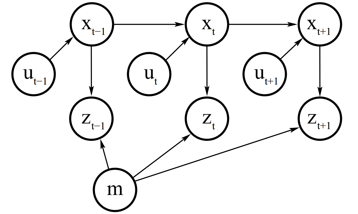
A Bayes filter can be represented as the factor graph shown in this figure, where $x_t$ denotes states, $u_t$ denotes control signal and $z_t$ denotes measurement, $m$ is the landmark.
Goal of Bayes Filter:
To estimate state $x$, given observation $z$ and control (action) $u$, which is to estimate the probability of a agent in state $x$, given $z$ and $u$
\begin{equation}
p(x | z , u)
\end{equation}
So the \textbf{belief} of the state $x$ at time step $t$, given observation and control (action) from $1:t$, is define as
\begin{equation}
bel(x_t) = p(x_t | z_{1:t}, u_{1:t})
\end{equation}
Sometimes it's useful to calculate a belief(posterior) before incorporating $z_t$, just after executing the control $u_t$, this belief is denoted as,
\begin{equation}
\overline{bel}(x_t) = p(x_t | z_{1:t-1}, u_{1:t})
\end{equation}
Derivation of Bayes filter
Aaccording to Bayes rule,
\begin{equation}
\begin{split}
p(x_t | z_{1:t}, u_{1:t}) &= p(x_t | z_{1:t}, u_{1:t}) \\
&= p(x_t | z_t, z_{1:t-1}, u_{1:t}) \\
&= \frac{p(z_t | x_t, z_{1:t-1}, u_{1:t}) p(x_t|z_{1:t-1}, u_{1:t})}
{p(z_t|z_{1:t-1}, u_{1:t})} \\
& = \eta p(z_t | x_t, z_{1:t-1}, u_{1:t}) p(x_t|z_{1:t-1}, u_{1:t}) \\
& \propto p(z_t | x_t, z_{1:t-1}, u_{1:t}) p(x_t|z_{1:t-1}, u_{1:t})
\end{split}
\end{equation}
Since term $p(z_t|z_{1:t-1}, u_{1:t})$ is a constant, we can denote it as $\frac{1}{\eta}$.
According to Markov assumption,
\begin{equation}
p(z_t | x_t, z_{1:t-1}, u_{1:t}) = p(z_t | x_t)
\end{equation}
thus we have,
\begin{equation}
\begin{split}
bel(x_t) &= p(x_t | z_{1:t}, u_{1:t}) \\
&= \eta p(z_t | x_t) p(x_t|z_{1:t-1}, u_{1:t}) \\
&= \eta p(z_t | x_t) \overline{bel}(x_t)
\end{split}
\end{equation}
According to theorem of total probability, we can link the belief of current state to the belief of previous state.
First let's assume that $x_t$ does not condition on $z_{1:t-1}$ and $u_{1:t}$, we have
\begin{equation}
p(x_t) = \int p(x_t|x_{t-1}) p(x_{t-1}) d x_{t-1}
\end{equation}
then we have the full expression,
\begin{equation}
\overline{bel}(x_t) = p(x_t|z_{1:t-1}, u_{1:t}) = \int p(x_t|x_{t-1}, z_{1:t-1}, u_{1:t}) p(x_{t-1}|z_{1:t-1}, u_{1:t}) d x_{t-1}
\end{equation}
Again, according to Markov assumption,
\begin{equation}
\begin{split}
\overline{bel}(x_t) &=
\int p(x_t|x_{t-1}, u_{t}) p(x_{t-1}|z_{1:t-1}, u_{1:t}) d x_{t-1} \\
&= \int p(x_t|x_{t-1}, u_{t}) p(x_{t-1}|z_{1:t-1}, u_{1:t-1}) d x_{t-1} \\
&= \int p(x_t|x_{t-1}, u_{t}) bel(x_{t-1}) d x_{t-1}
\end{split}
\end{equation}
Finally we have the two steps of Bayes filter: \\
Prediction step:
\begin{equation}
\overline{bel}(x_t) = \int p(x_t|x_{t-1}, u_{t}) bel(x_{t-1}) d x_{t-1}
\end{equation}
Correction step:
\begin{equation}
bel(x_t) = \eta p(z_t | x_t) \overline{bel}(x_t)
\end{equation}
Kalman Filter
Linear Kalman Filter
Linear Kalman Filter is really just a special case of Bayes Filter, where the state transition and measurement function are linear and follow Gaussian distribution. The state transition function is,
\begin{equation}
\mathbf{x}_t = \mathbf{A}_t \mathbf{x}_{t-1} + \mathbf{B}_t \mathbf{u_t} + \boldsymbol{\epsilon}_t
\end{equation}
The notations are explained as follows:
- $\mathbf{x}_t \sim \mathcal{N}(\boldsymbol{\mu_t}, \mathbf{\Sigma_t})$ denotes state vector at time $t$, and $\mathbf{x} \in \mathbb{R}^n$
- $\mathbf{u}_t$ denotes control vector at time $t$, and $\mathbf{u} \in \mathbb{R}^m$
- $\mathbf{A}$ denotes state transition model and $\mathbf{A} \in \mathbb{R}^{n \times n}$
- $\mathbf{B}$ denotes control model and $\mathbf{B} \in \mathbb{R}^{n \times m}$
- $\boldsymbol{\epsilon} \sim \mathcal{N}(\mathbf{0}, \mathbf{R})$ denotes process noise.
The posterior of state $\mathbf{x}_t$ after state transition is,
\begin{equation}
p(\mathbf{x}_t | \mathbf{u}_t, \mathbf{x}_{t-1}) = \frac{1}{\sqrt{(2 \pi)^n \text{det}(\mathbf{R}_t)}} \exp\left\{-\frac{1}{2}(\mathbf{x}_t - (\mathbf{A}_t \mathbf{x}_{t-1} + \mathbf{B}_t \mathbf{u_t}) )^{\top}\mathbf{R}_t^{-1}(\mathbf{x}_t - (\mathbf{A}_t \mathbf{x}_{t-1} + \mathbf{B}_t \mathbf{u_t}))\right\}
\end{equation}
Besides transition, we also need to have a measurement process. The measurement function is,
\begin{equation}
\mathbf{z}_t = \mathbf{C}_t \mathbf{x}_t + \boldsymbol{\delta}_t
\end{equation}
where $\boldsymbol{\delta}_t \sim \mathcal{N}(\mathbf{0}, \mathbf{Q}_t)$ is the measurement noise.
The posterior after measurement is
\begin{equation}
p(\mathbf{z}_t | \mathbf{x}_t) = \frac{1}{\sqrt{(2 \pi)^n \text{det}(\mathbf{Q}_t)}} \exp\left\{-\frac{1}{2}(\mathbf{z}_t - \mathbf{C}_t \mathbf{x}_t )^{\top}\mathbf{Q}_t^{-1}(\mathbf{z}_t - \mathbf{C}_t \mathbf{x}_t)\right\}
\end{equation}
Our goal is to find the Gaussian distribution of the state vector, which means finding its mean $\boldsymbol{\mu}_t$ and covariance matrix $\mathbf{\Sigma}_t$, based on the state transition function and measurement function.
The steps of Kalman filter algorithm are:
1. First, update \textbf{belief} of state $\mathbf{x}_t$ with state transition model:
\begin{equation}
\begin{split}
\hat{\boldsymbol{\mu}}_t = \mathbf{A}_t \boldsymbol{\mu}_{t-1} + \mathbf{B}_t \mathbf{u_t} \\
\hat{\mathbf{\Sigma}}_t = \mathbf{A}_t \mathbf{\Sigma}_{t-1}\mathbf{A}_t + \mathbf{R}_t
\end{split}
\end{equation}
2. Compute \textbf{Kalman Gain} (which tells us the extent to which we should incorporate sensor measurement $\mathbf{z}_t$ into state update) :
\begin{equation}
\begin{split}
\mathbf{K}_t = \hat{\mathbf{\Sigma}}_t \mathbf{C}_t^{\top} (\mathbf{C}_t \hat{\mathbf{\Sigma}}_t \mathbf{C}_t + \mathbf{Q}_t)^{-1}
\end{split}
\end{equation}
3. Update belief of $\mathbf{x}_t$ with measurement model:
\begin{equation}
\begin{split}
\boldsymbol{\mu}_t = \hat{\boldsymbol{\mu}}_t + \mathbf{K}_t (\mathbf{z}_t - \mathbf{C}_t \mathbf{x}_t ) \\
\mathbf{\Sigma}_t = (\mathbf{I} - \mathbf{K}_t \mathbf{C}_t)\hat{\mathbf{\Sigma}}_t
\end{split}
\end{equation}
Extended Kalman Filter
Reference
- Probalistic Robotics, by Sebastian Thrun, Wolfram Burgard, Dieter Fox
If you find this article helpful, please consider citing it in your research:
@article{Hu2026learnvslam,
  author = {Hu, Yafei},
  title = {Learning Visual SLAM: Filtering-based Methods for Visual SLAM},
  year = {2026}
}