Feature-based Visual Odometry
Two view geometry: Motion from 2D-2D correspondences
In this section we first talk about the very fundamental of geometric vision used in feature-based monocular visual odometry, that is two view geometry, which is used to solve motion from the 2D-2D image point correspondences.
Epipolar constraints
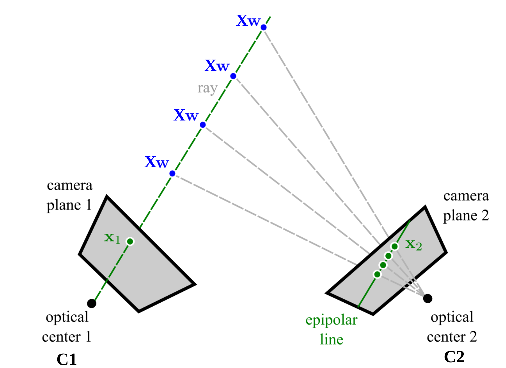
Epipolar line
The epipolar line is the $\textit{projection}$ of the $\textit{ray}$ that passes through the current image point $\mathbf{x}_1$ and the current optical center 1 $\mathbf{C}_1$ to another image plane.
And at the same time, the all possible 3D points $\mathbf{X}_w$ that might project to $\mathbf{x}_1$ should all lie on this ray. And all correspondences in camera 2 should lie on the epipolar line.
Here is an illustration of the epipolar line.
Epipoles
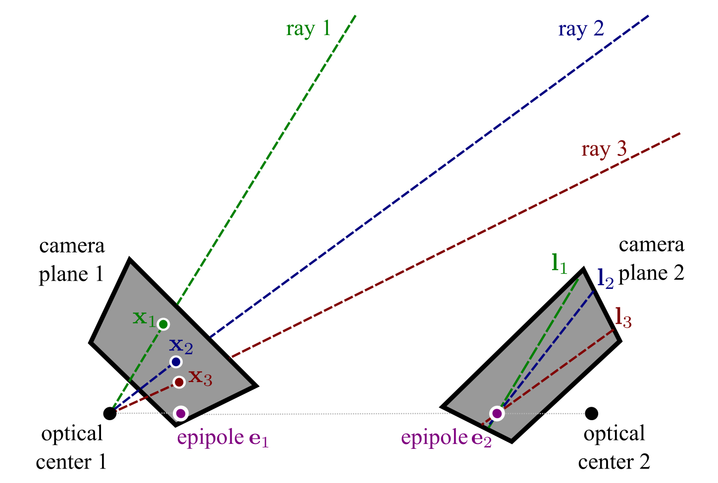
Another concept we need to introduce is the epipole. Epipole can be defined by in two ways:
1. The intersection points of the ray which connects two optical centers with the two image planes. In this case, the epipole in one image plane happens to be the projection of another optical center.
2. This also happens to be the intersection point of all epipolar lines in one image plane.
The following figure shows the epipole in two images.
The fundamental matrix and the essential matrix
Algebraic perspective
Given two correpondence points $\mathbf{x}_1$ and $\mathbf{x}_2$ in two images. They represent two projections of the same 3D point $\mathbf{X}_w$, and the two cameras are connected by a rigid body motion with rotation $\mathbf{R}$ and translation $\mathbf{t}$.
\begin{equation}
\tilde{\mathbf{x}_1} = \mathbf{K}_1[\mathbf{I}, \mathbf{0}]\tilde{\mathbf{X}}_w
\end{equation}
\begin{equation}
\tilde{\mathbf{x}_2} = \mathbf{K}_2[\mathbf{R}, \mathbf{t}]\tilde{\mathbf{X}}_w
\end{equation}
Note here $[\mathbf{R}, \mathbf{t}]$ denotes the transformation of camera 1 seen in camera 2's frame, or $\mathbf{T}_{21}$.
We can then represent the 3D point $\tilde{\mathbf{X}}_w$ in two camera coordinate frames $\mathcal{F}_{c1}$ and $\mathcal{F}_{c2}$, which are are $\tilde{\mathbf{X}}_{c1}$ and $\tilde{\mathbf{X}}_{c2}$, thus we have, with slight abuse of notation by removing $\tilde{.}$ symbol to represent the homogeneous coordinates.
\begin{equation}
\mathbf{X}_c = [\mathbf{I}, \mathbf{0}]\mathbf{X}_w = \mathbf{X}_w
\end{equation}
and
\begin{equation}
\mathbf{X}_{c2} = [\mathbf{R}, \mathbf{t}]\mathbf{X}_w = [\mathbf{R}, \mathbf{t}]\mathbf{X}_c
\end{equation}
So we have
\begin{equation}
\mathbf{X}_{c2} = \mathbf{R}\mathbf{X}_{c1} + \mathbf{t}
\label{eq:Xc2_Xc1_motion}
\end{equation}
This equation connects 3D corespondences $\mathbf{X}_{c1}$ and $\mathbf{X}_{c2}$ and their relative motion $\mathbf{R}$ and $\mathbf{t}$.
we then apply a small trick to the above equation, which is to cross product the left and right side of the equation with translation vector $\mathbf{t}$.
\begin{equation}
\mathbf{t} \times \mathbf{X}_{c2} = \mathbf{t} \times (\mathbf{R}\mathbf{X}_{c1}) + \mathbf{t} \times \mathbf{t}
\end{equation}
A basic property of cross product is that,
\begin{equation}
\mathbf{a} \times \mathbf{a} = ||\mathbf{a}|| ||\mathbf{a}|| \sin(0) = \mathbf{0}
\end{equation}
so we have,
\begin{equation}
\mathbf{t} \times \mathbf{X}_{c2} = \mathbf{t} \times (\mathbf{R}\mathbf{X}_{c1})
\end{equation}
Rewrite the cross product in matrix form,
\begin{equation}
[\mathbf{t}_\times] \mathbf{X}_{c2} = [\mathbf{t}_\times] \mathbf{R}\mathbf{X}_{c1}
\end{equation}
multiply $\mathbf{X}_{c2}^\top$ on both sides,
\begin{equation}
\mathbf{X}_{c2}^\top [\mathbf{t}_\times] \mathbf{X}_{c2} = \mathbf{X}_{c2}^\top [\mathbf{t}_\times] \mathbf{R}\mathbf{X}_{c1}
\end{equation}
the cross product of $[\mathbf{t}_\times] \mathbf{X}_{c2}$ is perpendicular to both $\mathbf{t}$ and $\mathbf{X}_{c2}$, thus the dot product of $\mathbf{X}_{c2}^\top$ and $[\mathbf{t}_\times]\mathbf{X}_{c1}$ is zero, which gives us,
\begin{equation}
\mathbf{X}_{c2}^\top [\mathbf{t}_\times] \mathbf{X}_{c2} = 0
\end{equation}
Then we have,
\begin{equation}
\mathbf{X}_{c2}^\top [\mathbf{t}_\times] \mathbf{R}\mathbf{X}_{c1} = 0
\label{eq:Xc2_Xc1_motion_dot}
\end{equation}
At this point we reach to a relationship between 3D corespondences $\mathbf{X}_{c1}$ and $\mathbf{X}_{c2}$ in camera frame and their relative motion $\mathbf{R}$ and $\mathbf{t}$.
What we will do is to connect up the 2D corespondences $\mathbf{x}_1$ and $\mathbf{x}_2$ in image plane with the relative camera motion $\mathbf{R}$ and $\mathbf{t}$. But at first we will have to bring camera intrinsics into the picture.
Pinhole projection model gives us,
\begin{equation}
\mathbf{x}_1 = \mathbf{K}_1 \mathbf{X}_{c1}
\end{equation}
\begin{equation}
\mathbf{x}_2 = \mathbf{K}_2 \mathbf{X}_{c2}
\end{equation}
substitute back to equation \ref{eq:Xc2_Xc1_motion_dot}, we have,
\begin{equation}
{(\mathbf{K}_2^{-1} \mathbf{x}_2)}^\top [\mathbf{t}_\times] \mathbf{R} (\mathbf{K}_1^{-1} \mathbf{x}_1) = 0
\end{equation}
hence,
\begin{equation}
{\mathbf{x}_2}^\top {({\mathbf{K}_2}^{-1})}^\top [\mathbf{t}_\times] \mathbf{R} {\mathbf{K}_1}^{-1} \mathbf{x}_1 = 0
\end{equation}
we define $\mathbf{F}$ as the $\textbf{fundamental matrix}$:
\begin{equation}
\mathbf{F} = {(\mathbf{K}_2^{-1})}^\top [\mathbf{t}_\times] \mathbf{R} \mathbf{K}_1^{-1}
\end{equation}
and define $\mathbf{E}$ as the $\textbf{essential matrix}$
\begin{equation}
\mathbf{E} = [\mathbf{t}_\times] \mathbf{R}
\end{equation}
so we finally reach to the desired relationship between 2D corespondences $\mathbf{x}_1$ and $\mathbf{x}_2$ and the camera relative motion $\mathbf{R}$ and $\mathbf{t}$,
\begin{equation}
{\mathbf{x}_2}^\top \mathbf{F} \mathbf{x}_1 = 0
\end{equation}
The relationships between $\mathbf{E}$ and $\mathbf{F}$ are obvious,
\begin{equation}
\mathbf{F} = {(\mathbf{K}_2^{-1})}^\top \mathbf{E} \mathbf{K}_1^{-1}
\end{equation}
\begin{equation}
\mathbf{E} = \mathbf{K}_2^\top \mathbf{F} \mathbf{K}_1
\end{equation}
An important property of $\mathbf{F}$ and $\mathbf{E}$ is that, they are only defined up to a scale, which means,
\begin{equation}
\begin{aligned}
{\mathbf{x}_2}^\top \mathbf{F} \mathbf{x}_1 = {\mathbf{x}_2}^\top (\alpha \mathbf{F}) \mathbf{x}_1 = 0
\end{aligned}
\end{equation}
where $\alpha$ is a arbitrary scalar. This reduces the DoF of $\mathbf{F}$ from 9 to 8.
Geometric perspective
Now we explain the geometric meaning of $\mathbf{F}$ and connect it up with the epipolar constraints we introduced in the previous section.
The algebraic representation of epipolar lines in two image planes are actually,
\begin{equation}
\mathbf{l}_2 = \mathbf{F} \mathbf{x}_1 \text{ and } \mathbf{l}_1 = \mathbf{F}^\top \mathbf{x}_2
\end{equation}
Next we will show why this is the case.
Substitute the epipolar line equation back to the defination of $\mathbf{F}$, we have,
\begin{equation}
\mathbf{x}_2^\top \mathbf{l}_2 = 0
\end{equation}
Recall the defination of a lone function
\begin{equation}
\mathbf{x}^\top \mathbf{l} = ax_2 + by_2 + c = 0
\end{equation}
where $a$, $b$ and $c$ are the coefficients of the line $\mathbf{l}$.
So this literally means image point $\mathbf{x}_2 = [x_2, y_2, 1]^\top$ lies on the epipolar line $\mathbf{l}_2$.
epipole $\mathbf{e}'$ is also on $\mathbf{l}'$, so we have
\begin{equation}
\mathbf{e}_2^\top \mathbf{l}_2 = 0
\end{equation}
\begin{equation}
\mathbf{e}_2^\top \mathbf{F} \mathbf{x}_1 = 0
\end{equation}
To make the above equation always true, we have to make sure that $\mathbf{e}_2$ is in the $\textbf{left nullspace}$ of $\mathbf{F}$.
\begin{equation}
\mathbf{e}_2^\top \mathbf{F} = 0
\end{equation}
We do no want the above epipole solution to be always $\mathbf{0}$, which is a trivial solution, or a trivial nullspace of $\mathbf{F}$. Thus we need to make sure the nullspace of $\mathbf{F}$ is not trivial. A matrix with a non-trival nullspace is a singular matrix and is not a full-rank matrix. Thus fundamental matrix (also essential matrix) is a singular matrix, $\det(\mathbf{F}) = 0$. In fact $\mathbf{F}$ is only of rank 2, which further reduce its DoF from 8 to 7.
Also recall the defination of null space for a matrix $\mathbf{A}$:
Let $\mathbf{A} \in \mathbb{R}^{m\times n}$.
The right nullspace is,
\begin{equation}
\mathcal{N}_R(\mathbf{A})
= \{\, \mathbf{x} \in \mathbb{R}^n \;\mid\; \mathbf{A}\mathbf{x} = \mathbf{0} \,\}.
\end{equation}
These are the $\textit{column vectors that get mapped to zero by $\mathbf{A}$}$.
left nullspace is,
\begin{equation}
\mathcal{N}_L(\mathbf{A})
= \{\, \mathbf{y} \in \mathbb{R}^m \;\mid\; \mathbf{y}^\top \mathbf{A} = \mathbf{0}^\top \,\}.
\end{equation}
8-point algorithm
Next we introduce a pratical algorithm to solve the essential matrix. We would need at least 8 correspondences to solve for $\mathbf{F}$ due to its scale ambiguity. This is where the classic 8-point algorithm comes in.
If we observe in further, we can find essential matrix $\mathbf{E}$ actually only has 5 DoF. Since $\mathbf{E} = [\mathbf{t}_\times] \mathbf{R}$ depends on $\mathbf{R}$ and $\mathbf{t}$, which only has 3 DoF, respectively. In total this gives us 6, and then we take 1 DoF off due to the scale ambiguity. And in fact, there's also a 5-point algorithm to solve for $\mathbf{E}$ with only 5 correspondences.
The reason we usually choose not to use 7 correspondences for $\mathbf{F}$, or 5 correspondences for $\mathbf{E}$ is that, usually we have more than 8 correspondences in practice and 8 point algorithm is simple and usually more stable.
And here we will introduce the 8-point algorithm to solve for $\mathbf{F}$.
Write the fundamental matrix in matrix form,
\begin{equation}
\begin{bmatrix}
x_1 & y_1 & 1
\end{bmatrix}
\begin{bmatrix}
f_1 & f_2 & f_3 \\
f_4 & f_5 & f_6 \\
f_7 & f_8 & f_9
\end{bmatrix}
\begin{bmatrix}
x_2 \\ y_2 \\ 1
\end{bmatrix}
= 0
\end{equation}
multiply on both sides, we have,
\begin{equation}
x_1 x_2 f_1 + x_1 y_2 f_4 + x_1 f_7 +
y_1 x_2 f_2 + y_1 y_2 f_5 + y_1 f_8 +
x_2 f_3 + y_2 f_6 + f_9 = 0
\end{equation}
we then have a general system of linear equations with $m$ correspondences,
\begin{equation}
\begin{bmatrix}
x^1_1 x^1_2 & x^1_1 y^1_2 & x^1_1 & y^1_1 x^1_2 & y^1_1 y^1_2 & y^1_1 & x^1_2 & y^1_2 & 1 \\
\vdots & \vdots & \vdots & \vdots & \vdots & \vdots & \vdots & \vdots & \vdots \\
x^M_1 x^M_2 & x^M_1 y^M_2 & x^M_1 & y^M_1 x^M_2 & y^M_1 y^M_2 & y^M_1 & x^M_2 & y^M_2 & 1
\end{bmatrix}
\begin{bmatrix}
f_1 \\ f_4 \\ f_7 \\ f_2 \\ f_5 \\ f_8 \\ f_3 \\ f_6 \\ f_9
\end{bmatrix}
= 0
\end{equation}
\begin{equation}
\mathbf{A} \mathbf{f} = 0
\end{equation}
then we use $m=8$ correspondences to solve for $\mathbf{F}$ with SVD.
\begin{equation}
\mathbf{A} = \mathbf{U}_A \mathbf{S}_A \mathbf{V}_A^\top
\end{equation}
The solution of $\mathbf{f}$ is the singular vector corresponding to smallest singular value of matrix $\mathbf{A}$, hence the last column of $\mathbf{V}_A$.
Exactly the same algorithm can be used to solve for $\mathbf{E}$ if we first normalize the correspondences with the camera intrinsics.
Solve motion from essential matrix
It is obvious that the trasnlation vector $\mathbf{t}$ is hidden in the essential matrix $\mathbf{E}$.
In fact,
\begin{equation}
[\mathbf{t}]_\times \mathbf{R} (-\mathbf{R}^\top \mathbf{t}) = - [\mathbf{t}]_\times \mathbf{t} = \mathbf{0}
\end{equation}
This means $ -\mathbf{R}^\top \mathbf{t} $ is in the right nullspace of $\mathbf{E}$.
\begin{equation}
\mathbf{E}^\top \mathbf{t} = \mathbf{R}^\top [\mathbf{t}]_\times^\top \mathbf{t} = \mathbf{R}^\top (- [\mathbf{t}]_\times) \mathbf{t} = \mathbf{0}
\end{equation}
This means $\mathbf{t}$ is in the left nullspace of $\mathbf{E}$.
Let's pause for a moment and think what $-\mathbf{R}^\top \mathbf{t}$ and $\mathbf{t}$ is. By definition, $\mathbf{t}$ is the camera 1's center seen in camera 2's frame.
The transformation which denotes camera 1's frame seen in camera 2's frame is $[\mathbf{R}, \mathbf{t}]$. Inversely, the transformation which denotes camera 2's frame seen in camera 1's frame is $[\mathbf{R}^\top, -\mathbf{R}^\top \mathbf{t}]$. Thus the left and right nullspaces of $\mathbf{E}$ happens to be the translation seen each of the camera frames.
If we apply camera intrinsics $\mathbf{K}_2$, epipole $\mathbf{e}_2$, which is the projection of camera 1's center in camera 2's image plane, is simply
\begin{equation}
\mathbf{e}_2 = \mathbf{K}_2 \mathbf{t}
\end{equation}
From the previous conclusion we know $\mathbf{e}_2$ is in the left nullspace of $\mathbf{F}$, and we just concluded that $\mathbf{t}$ is in the left nullspace of $\mathbf{E}$. Here it's all connected again. Trivially we can also verify the case for $\mathbf{e}_1$.
We introduce a Proposition here for the SVD of skew-symmetric matrix $[\mathbf{t}]_\times$. $[\mathbf{t}]_\times$ has singular values
\begin{equation}
(\,\|\mathbf{t}\|, \; \|\mathbf{t}\|, \; 0 \,),
\end{equation}
The SVD of $[\mathbf{t}]_\times$ is,
\begin{equation}
[\mathbf{t}]_\times = \mathbf{U} diag(|||\mathbf{t}||, ||\mathbf{t}||, 0) \mathbf{Z} \mathbf{U}^\top
\quad \text{where} \quad
\mathbf{Z} =
\begin{bmatrix}
0 & 1 & 0 \\
-1 & 0 & 0 \\
0 & 0 & 1
\end{bmatrix}
\end{equation}
The third column $\mathbf{u}_3$ of $\mathbf{U}$ spans the left nullspace, hence $\mathbf{u}_3 \parallel \mathbf{t}$.
There are two possible solutions for $\mathbf{t}$,
\begin{equation}
\mathbf{t}_1 = \mathbf{u}_3
\qquad
\mathbf{t}_2 = - \mathbf{u}_3
\end{equation}
(end of Proposition)
Since if the sign of $\mathbf{t}$ is flipped, the sign of $\mathbf{E}$ is also flipped, but the relationship $\mathbf{x}_2^\top \mathbf{E} \mathbf{x}_1 = 0$ still holds.
Substitute the SVD of $[\mathbf{t}]_\times$ back to $\mathbf{E}$, we have,
\begin{equation}
\begin{aligned}
\mathbf{E} &= \mathbf{U} \mathrm{diag}(||\mathbf{t}||, ||\mathbf{t}||, 0) \mathbf{Z} \mathbf{U}^\top \mathbf{R}
\end{aligned}
\end{equation}
set $\mathbf{Z} \mathbf{U}^\top \mathbf{R} = \mathbf{V}^\top$, it then gives the SVD form of $\mathbf{E}$. Previously we know that the rank of $\mathbf{E}$ is 2, and now we prove that it does have two singular values thus the rank is 2.
The third column $\mathbf{v}_3$ of $\mathbf{V}$ spans the right nullspace of $\mathbf{E}$, hence $\mathbf{v}_3 \parallel - \mathbf{R}^\top \mathbf{t}$.
Then we can solve $\mathbf{R}$ as,
\begin{equation}
\mathbf{R} = \mathbf{U} \mathbf{Z}^+ \mathbf{V}^\top = \mathbf{U} \mathbf{Z}^\top \mathbf{V}^\top
\end{equation}
$\mathbf{Z}^+$ is the pseudoinverse of $\mathbf{Z}$ since $\mathbf{Z}$ is a singular matrix and it happens to be $\mathbf{Z}^\top$.
Also, there are two possible solutions for $\mathbf{R}$,
\begin{equation}
\mathbf{R}_1 = \mathbf{U} \mathbf{Z} \mathbf{V}^\top, \quad \mathbf{R}_2 = \mathbf{U} \mathbf{Z}^\top \mathbf{V}^\top,
\end{equation}
Since if $\mathbf{t}$ is flipped, we use $\mathrm{diag}(-||\mathbf{t}||, -||\mathbf{t}||, 0)$ instead of $\mathrm{diag}(||\mathbf{t}||, ||\mathbf{t}||, 0)$, $\mathbf{R} = \mathbf{U} \mathbf{Z} \mathbf{V}^\top$.
To conlcusion, we have 4 possible solutions for transformation $[\mathbf{R}, \mathbf{t}]$,
\begin{equation}
(\mathbf{R}_1, \mathbf{t}_1), \quad (\mathbf{R}_1, \mathbf{t}_2), \quad (\mathbf{R}_2, \mathbf{t}_1), \quad (\mathbf{R}_2, \mathbf{t}_2)
\end{equation}
Let's discuss the relationship between the two solutions of $\mathbf{R}$ and $\mathbf{t}$. $\mathbf{t}_1$ and $\mathbf{t}_2$ are just same vectors with opposite directions. While for $\mathbf{R}_1$ and $\mathbf{R}_2$ they have this relationship:
\begin{equation}
\mathbf{R}_1 = \mathbf{U} \mathbf{Z} \mathbf{V}^\top = \mathbf{U} \mathbf{Z}^\top \mathbf{V}^\top (\mathbf{V} \mathbf{Z} \mathbf{Z} \mathbf{V}^\top) = \mathbf{R}_2 (\mathbf{V} \mathbf{Z} \mathbf{Z} \mathbf{V}^\top)
\end{equation}
Here we have a interesting matrix $\mathbf{V} \mathbf{Z} \mathbf{Z} \mathbf{V}^\top$, the inner part of this matrix is,
\begin{equation}
\mathbf{Z} \mathbf{Z} = \begin{bmatrix}
-1 & 0 & 0 \\
0 & -1 & 0 \\
0 & 0 & 1
\end{bmatrix}
\end{equation}
which is a rotation matrix that flips $x$ and $y$ axes, in the computer vision coordinate convention, this actually is a clockwise rotation of $180$ degrees around the $z$ axis.
So what about $\mathbf{V} \mathbf{Z} \mathbf{Z} \mathbf{V}^\top$? We need to bring another concept called $\textit{conjugated rotation}$. It changes the original rotation axis, which is $z$ axis (last axis) in the local camera frame, for $\mathbf{Z} \mathbf{Z}$, to the $z$-alike axis of $\mathbf{V}$, hence the axis represented by the last column of $\mathbf{V}$. What is the last column of $\mathbf{V}$? It represents the right nullspace of essential matrix $\mathbf{E}$, which is parallel to $-\mathbf{R}^\top \mathbf{t}$, camera 2's center seen in camera 1's frame. This is the baseline direction connecting two camera centers. Thus $\mathbf{V} \mathbf{Z} \mathbf{Z} \mathbf{V}^\top$ rotates camera by 180 degrees around the baseline direction. That's why in the figure below, the two solutions of $\mathbf{R}$ flipped around the baseline direction.
To disambiguate, we need to use the $\textit{cheirality test}$, which is to triangulate points using the two camera poses and select the solution where reconstructed 3D points have positive depth in both cameras. Triangulation will be introcuce in the next section.
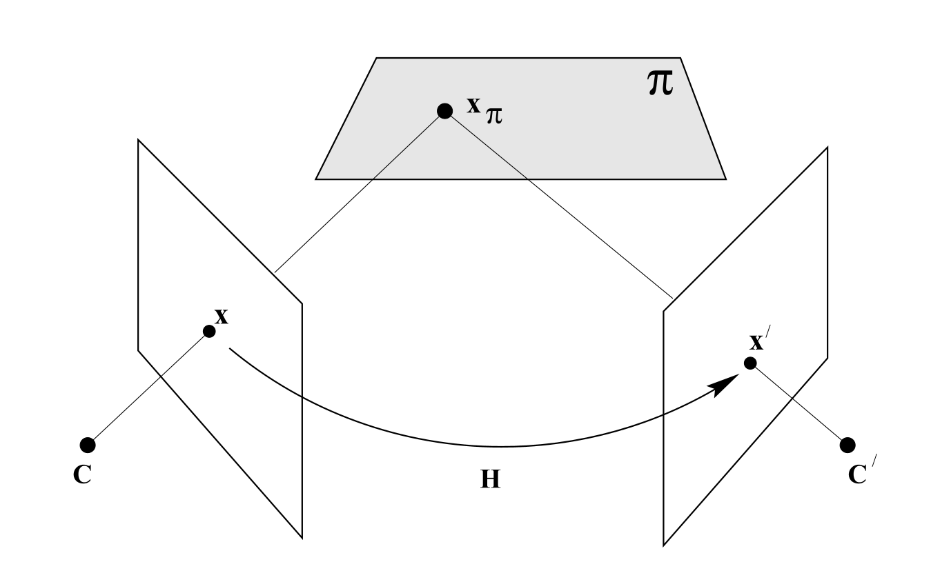
Planar Homography
When the 3D landmark points are in a plane, we can use homography to describe the relationship between 2D correspondences in two image planes.
\begin{equation}
\mathbf{n}^{\top}\mathbf{X} + d = 0.
\end{equation}
where $\mathbf{n}$ is the normal vector of the plane and $d$ is the distance from the origin to the plane.
Then we have,
\begin{equation}
-\,\frac{\mathbf{n}^{\top}\mathbf{X}}{d} = 1.
\end{equation}
Simply apply projection model, we have,
\begin{equation}
\begin{aligned}
\mathbf{x}_2 \ &= \mathbf{K}\!\left(\mathbf{R}\mathbf{X} + \mathbf{t}\right) \\
&= \mathbf{K}\!\left(\mathbf{R}\mathbf{X} + \mathbf{t}\cdot\left(-\,\frac{\mathbf{n}^{\top}\mathbf{X}}{d}\right)\right) \\
&= \mathbf{K}\!\left(\mathbf{R} - \frac{\mathbf{t}\mathbf{n}^{\top}}{d}\right)\mathbf{X} \\
&= \underbrace{\mathbf{K}\!\left(\mathbf{R} - \frac{\mathbf{t}\mathbf{n}^{\top}}{d}\right)\mathbf{K}^{-1}}_{\mathbf{H}}\ \mathbf{x}_1 .
\end{aligned}
\end{equation}
which gives the homography matrix $\mathbf{H}$ to connect the two image points. Note that similar to the essential matrix, the homography matrix is also only defined up to a scale.
\begin{equation}
\mathbf{x}_{2} = \mathbf{H} \mathbf{x}_{1}
\end{equation}
The homography matrix can be computed from 4 or more correspondences, with the same method as the essential matrix.
Next we talk about how to recover the motion from the homography matrix. The normalized homography matrix is defined as,
\begin{equation}
\hat{\mathbf{H}} = \mathbf{K}^{-1} \mathbf{H} \mathbf{K} = [\hat{\mathbf{h}}_{1}, \hat{\mathbf{h}}_{2}, \hat{\mathbf{h}}_{3}]
\end{equation}
A common trick is to assume that the the world frame align with the plane so that the Z axis of the 3D point on that plane is 0, then we have, hence $Z=0$. Then the projection can be written as,
\begin{equation}
\begin{aligned}
\mathbf{x} &= \mathbf{K}\,[\mathbf{r}_1 \ \mathbf{r}_2 \ \mathbf{r}_3 \ \mathbf{t}]
\begin{bmatrix}X \\ Y \\ 0 \\ 1\end{bmatrix} \\
&= \mathbf{K}\,[\mathbf{r}_1 \ \mathbf{r}_2 \ \mathbf{t}]
\begin{bmatrix}X \\ Y \\ 1\end{bmatrix} \\
&= \mathbf{H} \begin{bmatrix}X \\ Y \\ 1\end{bmatrix}
\end{aligned}
\end{equation}
The normalized homography in this case is:
$
\mathbf{\hat H} = \mathbf{K}^{-1}\mathbf{H}
$,
The first two columns of $\mathbf{R}$ and $\mathbf{t}$ can be directly obtained from $\mathbf{\hat H}$. But the third column of $\mathbf{R}$ is not directly obtained from $\mathbf{\hat H}$, and we ultilize the orthogonality of $\mathbf{R}$ to solve for it, which is,
\begin{equation}
\mathbf{r}_3 = \mathbf{r}_1 \times \mathbf{r}_2
\end{equation}
Triangulation and Reprojection Error
In this part we introduce the methods to compute the 3D landmark points from the 2D correspondences and the camera motion, which is often called triangulation.
In each image we have a measurement $\mathbf{x}_1 = \mathbf{P}_1 \mathbf{X} = \mathbf{K}_1 \mathbf{T}_{C_1W} \mathbf{X}$,
and$\mathbf{x}_2 = \mathbf{P}_2 \mathbf{X} = \mathbf{K}_2 \mathbf{T}_{C_2W} \mathbf{X}$, and these equations can be combined into a form
$\mathbf{A}\mathbf{X} = 0$, which is an equation linear in $\mathbf{X}$.
First the homogeneous scale factor is eliminated by a cross product to give three
equations for each image point, of which two are linearly independent.
For example, for the first image, with slight abuse of notation,
\begin{equation}
\begin{bmatrix}
x \\ y \\ 1
\end{bmatrix}
=
\begin{bmatrix}
\mathbf{p}_1^\top \\ \mathbf{p}_2^\top \\ \mathbf{p}_3^\top
\end{bmatrix}
\begin{bmatrix}
X \\ Y \\ Z
\end{bmatrix}
=
\begin{bmatrix}
\mathbf{p}_1^\top \mathbf{X} \\ \mathbf{p}_2^\top \mathbf{X} \\ \mathbf{p}_3^\top \mathbf{X}
\end{bmatrix}
\end{equation}
and apply $\mathbf{x} \times (\mathbf{P} \mathbf{X}) = 0$,
\begin{equation}
\begin{aligned}
x(\mathbf{p}_3^{\mathrm{T}}\mathbf{X}) - (\mathbf{p}_1^{\mathrm{T}}\mathbf{X}) &= 0 \\
y(\mathbf{p}_3^{\mathrm{T}}\mathbf{X}) - (\mathbf{p}_2^{\mathrm{T}}\mathbf{X}) &= 0 \\
x(\mathbf{p}_2^{\mathrm{T}}\mathbf{X}) - y(\mathbf{p}_1^{\mathrm{T}}\mathbf{X}) &= 0
\end{aligned}
\end{equation}
where $\mathbf{p}_i^{\mathrm{T}}$ are the rows of $\mathbf{P}$. The stack the above equations for both $x_1$ and $x_2$, we have a linear equation as,
\begin{equation}
\begin{bmatrix}
x_1\mathbf{p}_3^{\mathrm{T}} - \mathbf{p}_1^{\mathrm{T}} \\
y_1\mathbf{p}_3^{\mathrm{T}} - \mathbf{p}_2^{\mathrm{T}} \\
x_2\mathbf{p}_3^{\mathrm{T}} - \mathbf{p}_1^{\mathrm{T}} \\
y_2\mathbf{p}_3^{\mathrm{T}} - \mathbf{p}_2^{\mathrm{T}}
\end{bmatrix}
\mathbf{X}
=
\mathbf{A} \mathbf{X} = \mathbf{0}
\end{equation}
where two equations have been included from each image, giving a total of four equations
in four homogeneous unknowns. This is a redundant set of equations, since the solution
is determined only up to scale. The solution of $\mathbf{X}$ is the last column of $\mathbf{V}$ of the SVD of $\mathbf{A}$. This is called the DLT (Direct Linear Transform) method.
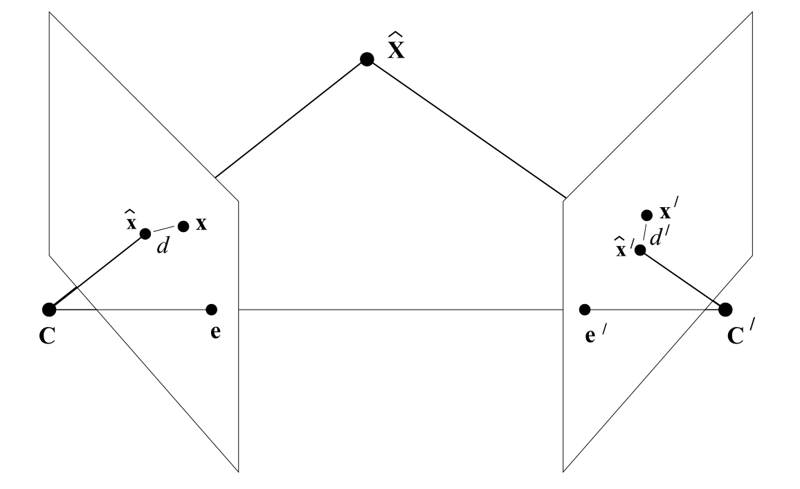
Besides solving the linear equation, triangulation can also be solved with a optimization method by minimizing the reprojection error.
\begin{equation}
\begin{aligned}
\hat{\mathbf{X}_{Wi}}^* = \arg \min_{\mathbf{X}_{Wi}} \left( \mathbf{e} \right) &= \arg \min_{\mathbf{X}_{Wi}} \frac{1}{2} \sum_{j=1}^{2} \left\| \mathbf{x}_i - \mathbf{P}_j \mathbf{X}_{Wi} \right\|_2^2 \\
&= \arg \min_{\mathbf{X}_{Wi}} \frac{1}{2} \sum_{j=1}^{2} \left\| \mathbf{x}_j - \pi(\mathbf{R}_j, \mathbf{t}_j, \mathbf{X}_{Wi}) \right\|_2^2 \\
\label{eq:reproj_error_triangulation}
\end{aligned}
\end{equation}
We usually use $\pi()$ to denote the projection function, please be reminded that the full projection is only up to a scale factor, but in the rest of the derivation we just igore the scale notation.
\begin{equation}
s_i \mathbf{x}_i = \mathbf{K} \mathbf{T}_{CW} \mathbf{X}_{Wi} .
\end{equation}
We need to find the derivate of the cost function with respect to the 3D point $\mathbf{X}_{Wi}$ to solve the optimization problem, simply apply the chain rule,
represent the point $\mathbf{X}_{Wi}$ in the camera frame as $\mathbf{X}_{Ci}$,
\begin{equation}
\mathbf{X}_{Ci}= \begin{bmatrix}
X' \\
Y' \\
Z'
\end{bmatrix}
\end{equation}
\begin{equation}
u = f_x \frac{X'}{Z'} + c_x,
\quad
v = f_y \frac{Y'}{Z'} + c_y.
\end{equation}
\begin{equation}
\frac{\partial \mathbf{e}}{\partial \mathbf{X}_{Wi}}
=
\frac{\partial \mathbf{e}}{\partial \mathbf{X}_{Ci}}
\frac{\partial \mathbf{X}_{Ci}}{\partial \mathbf{X}_{Wi}}.
\end{equation}
\begin{equation}
\mathbf{X}_{Ci} = (\mathbf{T}_{CW} \mathbf{X}_{Wi})_{1:3} = \mathbf{R X}_{Wi} + \mathbf{t}
\end{equation}
Going back to the reprojection error equation \ref{eq:reproj_error}, only the intrinsic matrix $\mathbf{K}$ is related to the 3D point $\mathbf{X}_{Ci}$, the derivative can be computed as,
\begin{equation}
\frac{\partial \mathbf{e}}{\partial \mathbf{X}_{Ci}}
=
-\begin{bmatrix}
\frac{\partial u}{\partial X'} & \frac{\partial u}{\partial Y'} & \frac{\partial u}{\partial Z'} \\
\frac{\partial v}{\partial X'} & \frac{\partial v}{\partial Y'} & \frac{\partial v}{\partial Z'}
\end{bmatrix}
=
-\begin{bmatrix}
\dfrac{f_x}{Z'} & 0 & -\dfrac{f_x X'}{Z'^2} \\
0 & \dfrac{f_y}{Z'} & -\dfrac{f_y Y'}{Z'^2}
\end{bmatrix}
\label{eq:partial_e_partial_X_Ci}
\end{equation}
Then the derivative of the cost function with respect to the 3D point in world frame $\mathbf{X}_{Wi}$ is,
\begin{equation}
\frac{\partial \mathbf{e}}{\partial \mathbf{X}_{Wi}}
=
-
\begin{bmatrix}
\dfrac{f_x}{Z'} & 0 & -\dfrac{f_x X'}{Z'^2} \\
0 & \dfrac{f_y}{Z'} & -\dfrac{f_y Y'}{Z'^2}
\end{bmatrix}
\mathbf{R}^\top
\end{equation}
PnP: Motion from 2D-3D correspondences
The PnP (Perspective-n-Point) problem is closely related to triangulation. It is to estimate the camera pose $\mathbf{R}$ and $\mathbf{t}$ from 3D-2D correspondences, $\mathbf{x}$ and $\mathbf{X}$ and we assume $\mathbf{X}$ is known and fixed.
In this problem we still apply the projection model, assume $\mathbf{K}$ is a identity matrix and with a slight abuse of notation,
\begin{equation}
\begin{bmatrix}
x \\ y \\ 1
\end{bmatrix}
=
[\mathbf{R} | \mathbf{t}]
\mathbf{X}
=
\begin{bmatrix}
\mathbf{p}_1^\top \\ \mathbf{p}_2^\top \\ \mathbf{p}_3^\top
\end{bmatrix}
\mathbf{X}
=
\begin{bmatrix}
\mathbf{p}_1^\top \mathbf{X} \\ \mathbf{p}_2^\top \mathbf{X} \\ \mathbf{p}_3^\top \mathbf{X}
\end{bmatrix}
\end{equation}
this is exactly the same as the case for triangulation, but here in PnP we are solve matrix $\mathbf{P}$ instead of $\mathbf{X}$.
So starts from the same equation as triangulation,
\begin{equation}
\mathbf{p}_1^{\top}\mathbf{X} - \mathbf{p}_3^{\top}\mathbf{X}\, x = 0,
\qquad
\mathbf{p}_2^{\top}\mathbf{X} - \mathbf{p}_3^{\top}\mathbf{X}\, y = 0 .
\end{equation}
we do a little rearrangement,
\begin{equation}
\mathbf{X}^{\top} \mathbf{p}_1 + 0 - \mathbf{X}^{\top} \mathbf{p}_3\, x = 0,
\qquad
0 + \mathbf{X}^{\top} \mathbf{p}_2 - \mathbf{X}^{\top} \mathbf{p}_3\, y = 0 .
\end{equation}
Stack the above equations for all correspondences $\{\mathbf{x}_i, \mathbf{X}_i\}$, we have a linear system as,
\begin{equation}
\begin{bmatrix}
\mathbf{X}_1^{\top} & \mathbf{0} & -x_1 \mathbf{X}_1^{\top} \\
\mathbf{0} & \mathbf{X}_1^{\top} & -y_1 \mathbf{X}_1^{\top} \\
\vdots & \vdots & \vdots \\
\mathbf{X}_N^{\top} & \mathbf{0} & -x_N \mathbf{X}_N^{\top} \\
\mathbf{0} & \mathbf{X}_N^{\top} & -y_N \mathbf{X}_N^{\top}
\end{bmatrix}
\begin{bmatrix}
\mathbf{p}_1 \\ \mathbf{p}_2 \\ \mathbf{p}_3
\end{bmatrix}
= \mathbf{0}.
\end{equation}
As a DLT solution to the above linear system, we will get a 12-dimensional vector stacking $\{\mathbf{p}_1, \mathbf{p}_2, \mathbf{p}_3\}$, or $[\hat{\mathbf{R}} | \hat{\mathbf{t}}]$ in matrix form. But remember the left part of the matrix is actually rotation matrix $\mathbf{R} \in \mathrm{SO}(3)$, and the directly solution may not satisfy the special property of $\mathbf{R}$, such as orthogonality and determinant 1. So we need to further constrain the solution to satisfy the special property of $\mathbf{R}$. To obtain a true rotation matrix, we project DLT estimation $\hat{\mathbf{R}}$ onto the
rotation manifold using the $\textit{polar decomposition}$.
Any nonsingular matrix $\hat{\mathbf{R}} \in \mathbb{R}^{3\times3}$ can
be decomposed as
\begin{equation}
\hat{\mathbf{R}} = \mathbf{R}\,\mathbf{S},
\end{equation}
where $\mathbf{R}$ is an orthogonal matrix and $\mathbf{S}$ is a symmetric positive-definite matrix.
The orthogonal factor $\mathbf{R}$ obtained from this decomposition
is precisely the minimizer of the Frobenius norm of the following objective function,
\begin{equation}
\mathbf{R}
= \arg\min_{\mathbf{R}\in O(3)}
\|\hat{\mathbf{R}} - \mathbf{R}\|_F .
\end{equation}
and the result can be computed as
\begin{equation}
\mathbf{R}
= \hat{\mathbf{R}}(\hat{\mathbf{R}}^\top \hat{\mathbf{R}})^{-\frac{1}{2}}
= (\hat{\mathbf{R}}\hat{\mathbf{R}}^\top)^{-\frac{1}{2}}\hat{\mathbf{R}}.
\end{equation}
Thus, the corrected rotation estimation is computed as
\begin{equation}
\mathbf{R} \;\leftarrow\;
(\hat{\mathbf{R}}\hat{\mathbf{R}}^\top)^{-\frac{1}{2}}\hat{\mathbf{R}}
\end{equation}
We can also address the PnP problem with a optimization method by minimizing the reprojection error w.r.t. the camera pose $\mathbf{T}_{CW} \in \mathrm{SE}(3)$. Apply the same optimization objective as the triangulation problem \ref{eq:reproj_error_triangulation},
\begin{equation}
\mathbf{T}_{CW}^* = \arg \min_{\mathbf{T}_{CW}} \left( \mathbf{e} \right) = \arg \min_{\mathbf{T}_{CW}} \left( \frac{1}{2} \sum_{i=1}^{n}\left\| \mathbf{x}_i - \mathbf{K} \mathbf{T}_{CW} \mathbf{X}_{Wi} \right\|_2^2 \right)
\label{eq:reproj_error}
\end{equation}
Take the derivative of the reprojection error with respect to the small perturbation $\boldsymbol{\xi} \in \mathfrak{se}(3)$ of the pose $\mathbf{T}_{CW}$,
\begin{equation}
\frac{\partial \mathbf{e}}{\partial \boldsymbol{\xi}}
=
\lim_{\delta \boldsymbol{\xi} \rightarrow 0}
\frac{
\mathbf{e}(\delta \boldsymbol{\xi} \oplus \boldsymbol{\xi}) - \mathbf{e}(\boldsymbol{\xi})
}{
\delta \boldsymbol{\xi}
}
=
\frac{\partial \mathbf{e}}{\partial \mathbf{X}_{Ci}}
\frac{\partial \mathbf{X}_{Ci}}{\partial \boldsymbol{\xi}}.
\end{equation}
Apply the pertubation model in $\mathrm{SE}(3)$ we previously derived, we have
\begin{equation}
\frac{\partial (\mathbf{T}_{CW} \mathbf{X}_{Wi})}{\partial \boldsymbol{\xi}}
=
(\mathbf{T}_{CW} \mathbf{X}_{Wi})^{\odot}
=
\begin{bmatrix}
\mathbf{I} & -(\mathbf{T}_{CW} \mathbf{X}_{Wi})^{\wedge} \\
\mathbf{0}^\top & \mathbf{0}^\top
\end{bmatrix}
=
\begin{bmatrix}
\mathbf{I} & -(\mathbf{X}_{Ci})^{\wedge} \\
\mathbf{0}^\top & \mathbf{0}^\top
\end{bmatrix}
\in \mathbb{R}^{4 \times 6}
\end{equation}
Multiply equation \ref{eq:partial_e_partial_X_Ci} and the above equation, we have
\begin{equation}
\frac{\partial \mathbf{e}}{\partial \delta \boldsymbol{\xi}} =
- \begin{bmatrix}
\frac{f_x}{Z'} & 0 & -\frac{f_x X'}{Z'^2} & -\frac{f_x X' Y'}{Z'^2} & f_x + \frac{f_x X'^2}{Z'^2} & -\frac{f_x Y'}{Z'} \\
0 & \frac{f_y}{Z'} & -\frac{f_y Y'}{Z'^2} & -f_y - \frac{f_y Y'^2}{Z'^2} & \frac{f_y X' Y'}{Z'^2} & \frac{f_y X'}{Z'}
\end{bmatrix}
\end{equation}
The optimization of the reprojection error with respect to the camera pose $\mathbf{T}_{CW}$ and 3D point $\mathbf{X}_{Wi}$ builds important foundation for the next important problem we will introduce, the bundle adjustment problem.
Extends to multiple views
In a real world scenario, the camera moves in the 3D space, and we need to compute the camera pose and 3D point in the world frame for each frame or slected frames. In pure visual odometry, using the first camera frame as the world frame is a common convention. We can just sequentially compute the relative motion between two consecutive frames and then get the trasnformation relatively to the initial frame. This process consists of the most basic part of the visual SLAM/odometry system, and is often called dead reckoning. Together with this sequentiall motion estimation, feature extraction, matching, and triangulation, we have the frontend of a visual SLAM system, also sometimes refered to as visual odometry. In real visual SLAM system, we often have more components such as bundle adjustment to refine the camera pose and 3D point, key-frame selection to reduce redundancy, and loop closure detection to correct the drift. Those components are usually refered to as the backend of visual SLAM system, which will be introduced in the next few sections.
References
- Visual SLAM: From Theory to Practice, by Xiang Gao, Tao Zhang, Qinrui Yan and Yi Liu
- Multiview Geometry in Computer Vision, by Richard Hartley and Andrew Zisserman
- Computer Vision 1st Edition, by Simon J. D. Prince
If you find this article helpful, please consider citing it in your research:
@article{Hu2026learnvslam,
  author = {Hu, Yafei},
  title = {Learning Visual SLAM: Feature-based Visual Odometry},
  year = {2026}
}