Direct Visual Odometry
Photometric loss and its optimization problem
the formulation of the photometric loss
Given two camera frames $\mathcal{F}_{C1}$ and $\mathcal{F}_{C2}$, or target and source respectively. We could find an implicit 2D correspondence $\mathbf{x}_{1}$ and $\mathbf{x}_{2}$ with estimated depth in the 2nd camera frame, denoted as $\hat{Z}_{2}$, and transform of these two frames $\hat{\mathbf{T}}_{12}$ (transform 3D point expressed in the 2nd frame to point expressed in the 1st frame).
Based on a estimated depth $\hat{Z_2}$, we can project the 2D point and get the estimated 3D point $\hat{\mathbf{X}}_{C2}$ in camera frame,
\begin{equation}
\hat{\mathbf{X}}_{C2} = \pi ^{-1} (\hat{Z_2}, \mathbf{K}, \mathbf{x}_{2}) = \hat{Z_2}\,\mathbf{K}^{-1}\ \mathbf{x}_{2} = [X_{2}, Y_{2}, Z_{2}]^\top
\end{equation}
Then transform the point based on estimated pose to the 1st frame,
\begin{equation}
\hat{\mathbf{X}}_{C1} = \hat{\mathbf{T}}_{12} \hat{\mathbf{X}}_{C2} = \hat{\mathbf{T}}_{12} \left( \hat{Z_2}\,\mathbf{K}^{-1}\ \mathbf{x}_{2} \right) = [X_{1}, Y_{1}, Z_{1}]^\top
\end{equation}
and then get the warped 2D image point,
\begin{equation}
\mathbf{x}_{wp} = \pi \left( \mathbf{K}, \hat{\mathbf{X}}_{C1} \right) = \frac{\mathbf{K} \hat{\mathbf{X}}_{C1}}{Z_{C1}} = \frac{ \mathbf{K} \hat{\mathbf{T}}_{12} \left(\hat{Z_2} \mathbf{K}^{-1} \mathbf{x}_{2} \right)}{\left[ \hat{\mathbf{T}}_{12} \left(\hat{Z_2} \mathbf{K}^{-1} \mathbf{x}_{2} \right) \right]_3}
\end{equation}
$\left[ \cdot \right]_3$ means the 3rd element of a vector.
If the estimated depth in ref frame $\hat{Z_2}$, and the estimated pose $\hat{\mathbf{T}}_{12}$ are all perfectly accurate, then the warped image point $\mathbf{x}_{wp}$ should exactly align with the 2D correpondence of $\mathbf{x}_{2}$, hence $\mathbf{x}_{1}$. But this is not the case, then we have an optimization problem to optimize $\hat{Z_2}$ and $\hat{\mathbf{T}}_{12}$, based on the pixel intensity of the points $\mathbf{x}_{wp}$ and $\mathbf{x}_{1}$, denoted as $I_{\mathrm{wp}}$, $I_{\mathrm{1}}$, respectively. The loss function is called $\textit{photometric loss}$, which is formulated as,
\begin{equation}
J = \frac{1}{N}\sum_{i=1}^{N}
\left\| I_{\mathrm{1}}(i) - I_{\mathrm{wp}}(i)\,\right\|^2 = \frac{1}{N}\sum_{i=1}^{N} \left\| e_i \right\|^2
\end{equation}
where $N$ denotes the total number of points.
For RGBD and stereo camera rig, it is easy to direct compute the depth map $\hat{Z_2}$ from the depth sensor. But for monocular cameras, the depth needs to be estimated.
pose optimization
We first derive the gradient of error term $e$ w.r.t pose, assuming constant depth $\hat{Z_2}$,
where,
\begin{equation}
\mathbf{x}_{2}= [u_2, v_2, 1 ]^\top
\qquad
\mathbf{x}_{1} = [u_1, v_1, 1 ]^\top
\end{equation}
Consider the left perturbation model of Lie algebra, using the first-order Taylor expansion:
Here we denote the transformation $\hat{\mathbf{T}}_{12}$,
\begin{equation}
e(\mathbf{\hat{T}_{12}}) = I_{\mathrm{1}}(\mathbf{x}_{1}) - I_{\mathrm{wp}}(\mathbf{x}_{wp})
\end{equation}
Then we derive the gradient of this error term w.r.t. the pose, but instead of computing the derivative on SE(3), we only do it in its lie algebra $\mathfrak{se}(3)$, hence,
\begin{equation}
\frac{\partial e}{\partial \delta \boldsymbol{\xi}}
= - \frac{\partial I_{wp}}{\partial \mathbf{x}_{wp}}
\frac{\partial \mathbf{x}_{wp}}{\partial \hat{\mathbf{X}}_{C1}}
\frac{\partial \hat{\mathbf{X}}_{C1}}{\partial \delta \boldsymbol{\xi}},
\end{equation}
where $\delta \boldsymbol{\xi} \in \mathfrak{se}(3)$ is the left disturbance of $\mathbf{\hat{T}}$, where
$\frac{\partial I_{wp}}{\partial \mathbf{x}_{wp}}$ is the grayscale gradient at pixel coordinate $\mathbf{x}_{wp}$.
$\frac{\partial \mathbf{x}_{wp}}{\partial \hat{\mathbf{X}}_{C1}}$ is the derivative of the projection equation with respect to the three-dimensional point in the camera frame. Let $\hat{\mathbf{X}}_{C2} = [X_2, Y_2, Z_2]^{\top}$:
\begin{equation}
\frac{\partial \mathbf{x}_{wp}}{\partial \hat{\mathbf{X}}_{C1}} =
\begin{bmatrix}
\frac{f_x}{Z_2} & 0 & -\frac{f_x X_2}{Z_2^2} \\
0 & \frac{f_y}{Z_2} & -\frac{f_y Y_2}{Z_2^2}
\end{bmatrix}.
\end{equation}
$\frac{\partial \hat{\mathbf{X}}_{C1}}{\partial \delta \boldsymbol{\xi}}$ is the derivative of the transformed three-dimensional point with respect to the transformation, which was introduced before as,
\begin{equation}
\frac{\partial \hat{\mathbf{X}}_{C1}}{\partial \delta \boldsymbol{\xi}} =
[\mathbf{I}, -(\hat{\mathbf{X}}_{C2})^{\wedge}].
\end{equation}
We can combine them together as:
\begin{equation}
\frac{\partial \mathbf{x}_{wp}}{\partial \delta \boldsymbol{\xi}} =
\begin{bmatrix}
\frac{f_x}{Z_2} & 0 & -\frac{f_x X_2}{Z_2^2} & -\frac{f_x X_2 Y_2}{Z_2^2} & f_x + \frac{f_x X_2^2}{Z_2^2} & -\frac{f_x Y_2}{Z_2} \\
0 & \frac{f_y}{Z_2} & -\frac{f_y Y_2}{Z_2^2} & -f_y - \frac{f_y Y_2^2}{Z_2^2} & \frac{f_y X_2 Y_2}{Z_2^2} & \frac{f_y X_2}{Z_2}
\end{bmatrix}.
\end{equation}
This $2 \times 6$ matrix also appeared in the previous post. Therefore, we derive the Jacobian of residual with respect to Lie algebra as:
\begin{equation}
\mathbf{J}_{\boldsymbol{\xi}} = - \frac{\partial I_{wp}}{\partial \mathbf{x}_{wp}}
\frac{\partial \mathbf{x}_{wp}}{\partial \delta \boldsymbol{\xi}}.
\end{equation}
Based on the Gauss-Newton method, the incremental update of the pose is given as,
\begin{equation}
\mathbf{J}_{\boldsymbol{\xi}}^\top \mathbf{J}_{\boldsymbol{\xi}} \delta \boldsymbol{\xi} = \mathbf{J}_{\boldsymbol{\xi}}^\top e \\
\end{equation}
the incremental update is solved as,
\begin{equation}
\begin{aligned}
\delta \boldsymbol{\xi} &= (\mathbf{J}_{\boldsymbol{\xi}}^\top \mathbf{J}_{\boldsymbol{\xi}} )^{-1} \mathbf{J}_{\boldsymbol{\xi}} ^\top e \\
&= (\mathbf{H}_{\boldsymbol{\xi}})^{-1} \mathbf{J}_{\boldsymbol{\xi}}^\top e
\end{aligned}
\end{equation}
where $\mathbf{H}_{\boldsymbol{\xi}}$ is the approximated Hessin.
Following the left-multiplicative composition rule, The pose is then updated as,
\begin{equation}
\hat{\mathbf{T}}_{k+1} = \exp \left( (\delta \boldsymbol{\xi})^\wedge \right) \hat{\mathbf{T}}_{k}
\end{equation}
where $k$ is the iteration step.
This Jacobian is used in to gradient-based optimization problem to update the camera pose. From the above equation we can see that that gradient is 0 when the pixel gradient is 0, which means feature-less regions will have 0 gradient, this explain why classical direct methods like LSD-SLAM and DSO choose image regions with rich textures.
Depth optimization
Next let's discuss how depth is estimated, the estimation method may vary in different approaches. And we will discuss two approches here in this tutorial that displayed in 1. SVO, and 2. Direct Sparse Odometry (DSO). In practice, for numerical stability, it's often use the inverse depth, or disparity $d = \frac{1}{Z}$ to perform the computation.
Bayesian optimization
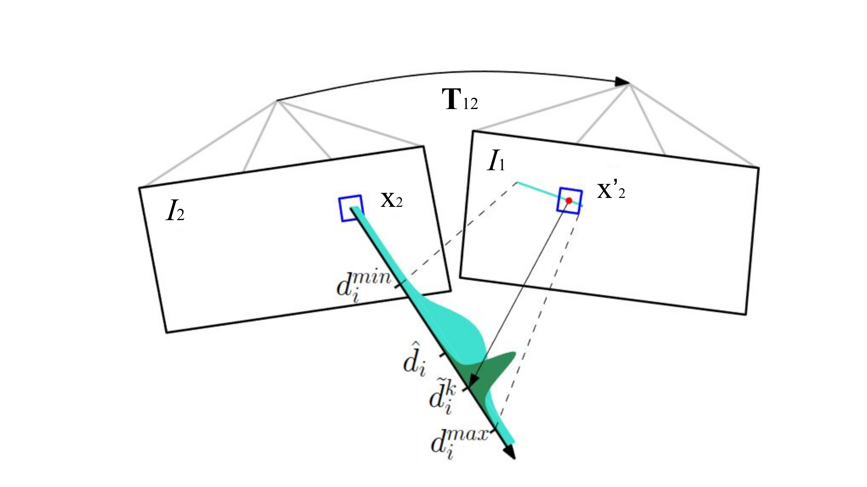
The first approach is to compute a ray given one 2D point in frame $\mathcal{F}_{C2}$, denoted as $\mathbf{x}_2$, and previous optimized pose $\hat{\mathbf{T}}_{12}$. The projection of this ray, is the epipolar line in frame $\mathcal{F}_{C1}$. The depth is initialized with in a range $\left[d_i^{\min}, d_i^{\max} \right]$.
\begin{equation}
p\!\left(d_i^{k} \mid d_i, \rho_i\right)
= \rho_i\, \mathcal{N} \left(d_i^{k};\, d_i, \tau_i^{2}\right)
+ (1-\rho_i)\, \mathcal{U} \left(d_i^{k};\, d_i^{\min}, d_i^{\max}\right),
\end{equation}
where $\rho_i$ is the probability that the measurement is an inlier. In this equation we use two distributions to model the depth uncertainty: Gaussian distribution $\mathcal{N}(d_i^k; d_i, \tau_i^2)$ meeans that if the measurement is an inlier, it should be close to the true depth $d_i$, with variance $\tau_i^2$; and a uniform distribution $\mathcal{U}(d_i^k; d_i^{\min}, d_i^{\max})$, meaning if the measurement is an outlier, it could be anywhere in the valid depth range. The variance term $\tau_i^2$ is computed by propagating a 1-pixel phometric matching error through the triangulation, which converts image-space uncertainty into depth-space uncertainty. The posterior of the depth $d_i$ is then updated recursively.
Gradient-based optimization
The SE(3) pose is optimized via gradient-based method like Gauss-Newton. The depth, can also be optimized in a similar way. Let's derive the gradient of the optimization objective with respect to the depth map $\hat{Z_2}$.
Following the similar chain rule:
\begin{equation}
\frac{\partial e}{\partial \hat{Z_2}} = -\frac{\partial I_{\text{wp}}}{\partial \mathbf{x}_{wp}} \cdot \frac{\partial \mathbf{x}_{wp}}{\partial \hat{\mathbf{X}}_{C1}} \cdot \frac{\partial \hat{\mathbf{X}}_{C1}}{\partial \hat{Z_2}} = \mathbf{J}_{\hat{Z}}
\end{equation}
The first two parts of the gradient $\frac{\partial e}{\partial \hat{Z_2}}$ has been discussed in the previous section. The derivative of $\hat{\mathbf{X}}_{C1}$ with respect to estimated depth in 2nd frame $\hat{Z}_2$. A search is then conducted for a patch on the epipolar line in the image 1 that has the highest correlation with the reference patch in image 2.
\begin{equation}
\frac{\partial \hat{\mathbf{X}}_{C1}}{\partial \hat{Z}_2}= \hat{\mathbf{T}}_{12} \mathbf{K}^{-1} \mathbf{x}_{2}
\end{equation}
Based on Gauss-Newton, the incremental update of depth is given as:
\begin{equation}
\mathbf{J}_{\hat{Z}}^\top \mathbf{J}_{\hat{Z}} \, \delta\hat{Z} = \mathbf{J}_{\hat{Z}}^\top \mathbf{e}
\end{equation}
\begin{equation}
\delta\hat{Z} = \left( \mathbf{J}_{\hat{Z}}^\top \mathbf{J}_{\hat{Z}} \right)^{-1} \mathbf{J}_{\hat{Z}}^\top \mathbf{e}
\end{equation}
The depth is then updated as:
\begin{equation}
\hat{Z}_{k+1} = \hat{Z}_k - \delta\hat{Z}
\end{equation}
Sparse Direct Visual Odometry
In sparse direct methods, we also optimize the camera pose to minimize the photometric error, but insteand of using the whole image or a alrge chunk of image, we only use points from the keypoint and optical flow tracking (e.g. KLT). Here the photometric error is the brightness error of the two pixels of $\mathbf{X}$ projrected to two images:
The previous introduced feature-based visual odometry methods are mostly always sparse due to the extraction of keypoint and point features in images. In sparse direct visual odometry, we also track sparse keypoints in images, but instead of using features, we use the pixel intensity values directly. This will apply the sparse optical flow we introcued previously, e.g. Lucas-Kanade method.
Dense Direct Visual Odometry
In a dense direct visual odometry, we ultilize the pixel intensity in the entire image. The first steps of direct VO is to have an initial guess of current reference depth map $\hat{Z_2}$ and camera pose $\hat{\mathbf{T}} = [\hat{\mathbf{R}},\hat{\mathbf{t}}]$. Then we wp the reference image to the target frame using the estimated camera pose and depth map, and compute the photometric loss between the warped image and the target image, to optimize the camera pose and depth map.
References
- Visual SLAM: From Theory to Practice, by Xiang Gao, Tao Zhang, Qinrui Yan and Yi Liu
- SVO: Fast Semi-Direct Monocular Visual Odometry, by Christian Forster, Matia Pizzoli, Davide Scaramuzza, ICRA 2014
- LSD-SLAM: Large-Scale Direct Monocular SLAM, by Jakob Engel and Thomas Schops and Daniel Cremers, ECCV 2014
- Direct Sparse Odometry, by Jakob Engel, Vladlen Koltun, Daniel Cremers, arXiv:1607.02565 2016
If you find this article helpful, please consider citing it in your research:
@article{Hu2026learnvslam,
  author = {Hu, Yafei},
  title = {Learning Visual SLAM: Direct Visual Odometry},
  year = {2026}
}