Cameras, Sensors and Projection Model
Pinhole Projection Model
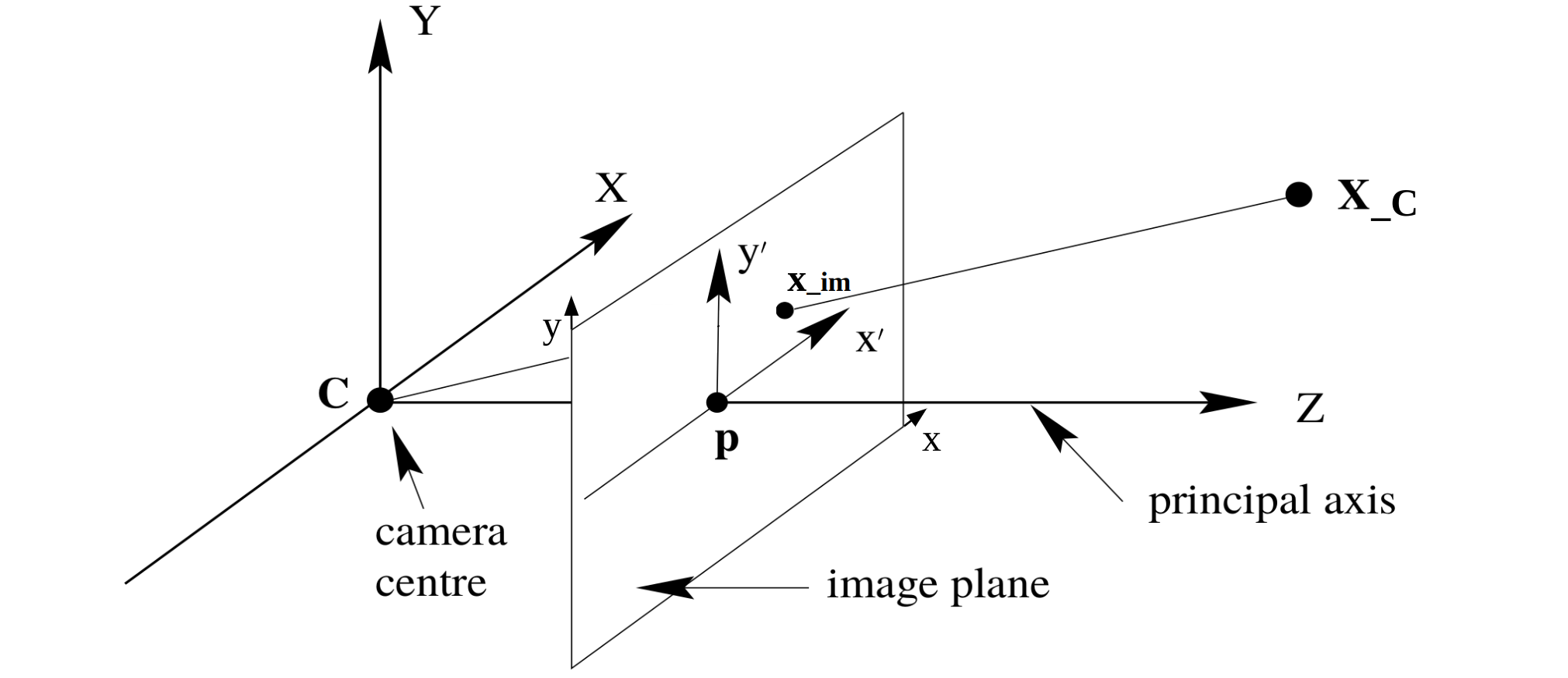
Pinhole camera projection model is the most common camera projection model. It is a simple model that projects a 3D point to a 2D image plane.
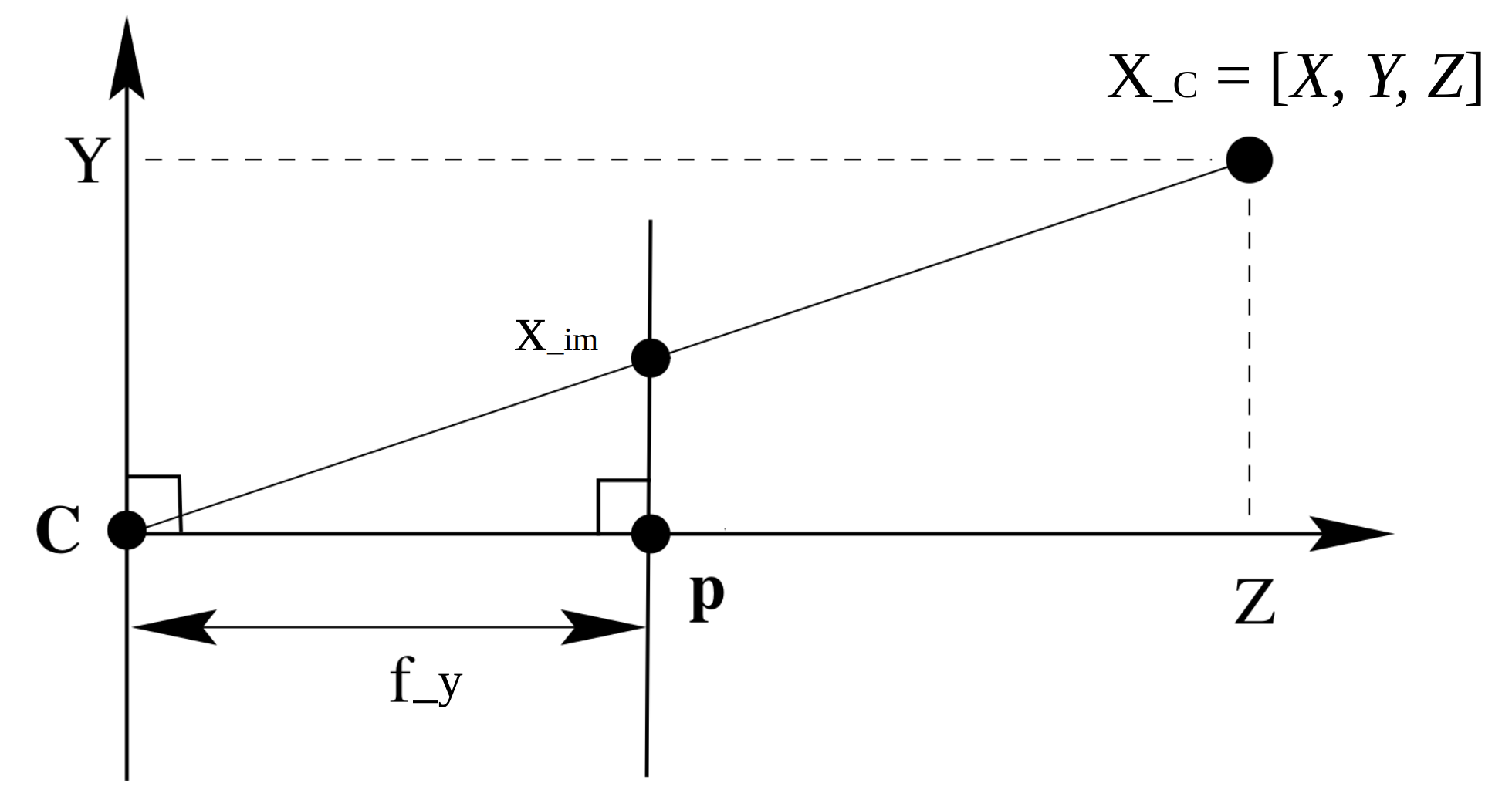
We first dicuss the projection of 3D points in camera coordinate system to 2D image points. Slice one place of the above 3D space,
With simple geometry rules, we find the camera intrinsic matrix as,
\begin{equation}
\frac{Z}{f_y} = \frac{Y}{y}
\quad
\quad
\frac{Z}{f_x} = \frac{X}{x}
\end{equation}
\begin{equation}
y = \frac{f_y Y}{Z}
\quad
\quad
x = \frac{f_x X}{Z}
\end{equation}
which is a mapping from 3D Euclidean space to 2D Euclidean space,
\begin{equation}
\begin{bmatrix}
X \\
Y \\
Z \\
\end{bmatrix}
\longrightarrow
\begin{bmatrix}
\frac{f_x X}{Z} \\
\\
\frac{f_y Y}{Z} \\
\end{bmatrix}
\end{equation}
considering the principal point, the final coordinate of the projected 3D point in camera coordinate system $X_c$ is, which is denoted as $x_i$
\begin{equation}
\mathbf{x}_i =
\begin{bmatrix}
u \\
v \\
\end{bmatrix}
=
\begin{bmatrix}
\frac{f_x X}{Z} + c_x\\
\\
\frac{f_y Y}{Z} + c_y\\
\end{bmatrix}
\end{equation}
\begin{equation}
\tilde {\mathbf{x}}_i
=
\begin{bmatrix}
u \\
v \\
1 \\
\end{bmatrix}
=
\begin{bmatrix}
\frac{f_x X}{Z} + c_x\\
\\
\frac{f_y Y}{Z} + c_y\\
\\
1 \\
\end{bmatrix}
\end{equation}
now we want to write it in matrix form,
\begin{equation}
\tilde {\mathbf{x}}_i = \mathbf{K} \mathbf{X}_C
\end{equation}
\begin{equation}
\begin{bmatrix}
f_x & 0 & c_x \\
0 & f_y & c_y \\
0 & 0 & 1 \\
\end{bmatrix}
\begin{bmatrix}
X \\
Y \\
Z \\
\end{bmatrix}
=
\begin{bmatrix}
f_x X + c_x Z \\
f_y Y + c_y Z \\
Z
\end{bmatrix}
=
Z
\begin{bmatrix}
f_x X \verb|/| Z + c_x \\
f_y Y \verb|/| Z + c_y \\
1
\end{bmatrix}
\end{equation}
$\mathbf{K}$ is camera intrinsic matrix
\begin{equation}
\mathbf{K} =
\begin{bmatrix}
f_x & 0 & c_x \\
0 & f_y & c_y \\
0 & 0 & 1 \\
\end{bmatrix}
\end{equation}
Generally, we want to have all of the coordinates in homogeneous coordinates, which gives
\begin{equation}
\tilde {\mathbf{x}}_i = \mathbf{K} \tilde {\mathbf{X}}_C =
\begin{bmatrix}
f_x & 0 & c_x & 0\\
0 & f_y & c_y & 0 \\
0 & 0 & 1 & 0\\
\end{bmatrix}
\begin{bmatrix}
X \\
Y \\
Z \\
1
\end{bmatrix}
\end{equation}
and matrix $\mathbf{T}_{CW}$ is the camera extrinsic matrix, which happens to be the inverse of $\mathbf{T}_{WC}$, the camera pose in world frame.
If we want to recover the 3D points in camera frame, we can try to back project the 3D image point by inversing the camera intrinsic matrix,
\begin{equation}
\begin{aligned}
\mathbf{X}_C &= \mathbf{K}^{-1} \tilde {\mathbf{x}}_i \\
&=
\begin{bmatrix}
\frac{1}{f_x} & 0 & -\frac{c_x}{f_x} \\
0 & \frac{1}{f_y} & -\frac{c_y}{f_y} \\
0 & 0 & 1
\end{bmatrix}
\begin{bmatrix}
u \\
v \\
1
\end{bmatrix} \\
&=
\begin{bmatrix}
\frac{u - c_x}{f_x} \\
\frac{v - c_y}{f_y} \\
1
\end{bmatrix}
\end{aligned}
\end{equation}
What is missing comparing with the original 3D points? We need the depth information $Z$, multiply the depth information we obtain,
\begin{equation}
\mathbf{X}_C =
\begin{bmatrix}
\frac{(u - c_x)Z}{f_x} \\
\frac{(v - c_y)Z}{f_y} \\
Z
\end{bmatrix}
\end{equation}
How to get the depth information? We will need at least two views, or specific depth sensors.
The full projection model also includes the rigid body transformation of camera frame seen from the world frame, denoted as $\mathbf{T}_{WC}$. But in camera projection model, we trasnform a 3D point in world frame to a 3D point in camera frame, making the convention using $\mathbf{T}_{CW}$ to denote the camera extrinsic matrix.
\begin{equation}
\tilde{\mathbf{X}}_C = \mathbf{T}_{CW} \tilde{\mathbf{X}}_W
=
\tilde{\mathbf{X}}_W
\end{equation}
here $\tilde{\mathbf{X}}_W$ is the 3D point in world frame in homogeneous coordinates.
Combine the camera intrinsic matrix and the camera extrinsic matrix, we get the full projection model,
\begin{equation}
\mathbf{x} = \mathbf{P} \mathbf{X}_W = \mathbf{K} \mathbf{T}_{CW} \tilde{\mathbf{X}}_W
\end{equation}
Camera Distortion Model
The real camera is usually not a perfect pinhole camera, it has some distortions. We model two common distortion models, the radial distortion and the tangential distortion.
Radial Distortion
The radial distortiono ccurs when the lens is not perfectly spherical. It is caused by the lens being too close to the image sensor.
it is modeled by parameters $k_1$, $k_2$, $k_3$ as,
\begin{equation}
x_{\text{distorted}} = x(1 + k_1 r^2 + k_2 r^4 + k_3 r^6) \\
y_{\text{distorted}} = y(1 + k_1 r^2 + k_2 r^4 + k_3 r^6)
\end{equation}
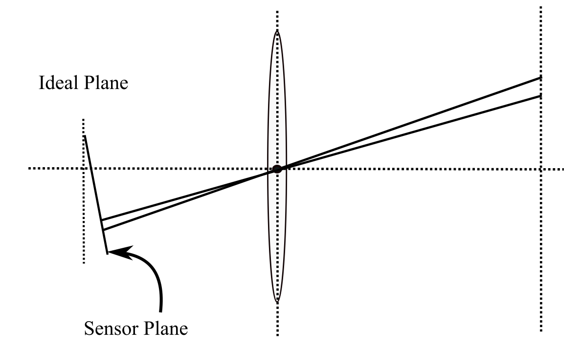
Tangential Distortion
The tangential distortion is caused by lens misalignment, hence not perfectly parallel to image plane. It is illustrated as the following figure.
The tangential distortion is modeled by parameters $p_1$ and $p_2$,
\begin{equation}
x_{\text{distorted}} = x + 2p_1 xy + p_2 (r^2 + 2x^2) \\
y_{\text{distorted}} = y + p_1 (r^2 + 2y^2) + 2p_2 xy
\end{equation}
Putting the two distortion models together, we get a joint model with 5 distortion coefficients,
\begin{equation}
\left\{
\begin{aligned}
x_{\text{distorted}} &= x(1 + k_1 r^2 + k_2 r^4 + k_3 r^6) + 2p_1 xy + p_2 (r^2 + 2x^2) \\
y_{\text{distorted}} &= y(1 + k_1 r^2 + k_2 r^4 + k_3 r^6) + p_1 (r^2 + 2y^2) + 2p_2 xy
\end{aligned}
\right.
\end{equation}
Stereo Camera and Stereo Matching
As we mentioned before, camera projection will lose the depth information. One way to recover the depth information is to use stereo cameras via a process called stereo matching. We will now derive the math model of stereo matching.
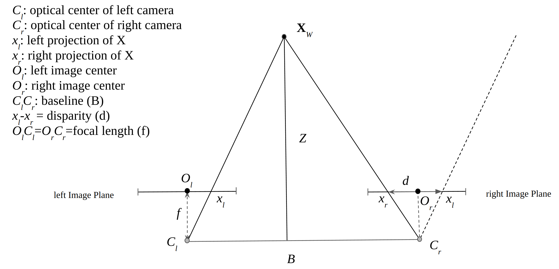
The key concepts of stereo matching are denoted as the following figure.
Based on simple geometry, we can find the the relationship of depth $Z$, disparity $d$, baseline $B$ and focal length $f$ as,
\begin{equation}
\begin{aligned}
\frac{d}{f} = \frac{B}{Z} \\
Z = \frac{B f}{d}
\end{aligned}
\end{equation}
where $d$ is the disparity, $B$ is the baseline, $f_x$ is the focal length, $Z$ is the depth. The disparity is the difference in the x-coordinates of the same point projected onto the two cameras.
Common Sensors used in Visual SLAM
Stereo Cameras
Many exsiting visual-(inertial) SLAM systems, such as ORB-SLAM3 and okvis2 can be used in the following commercial sensors. They are stereo cameras usually with a buit-in IMU inside them. Here is a table summarizing the sensors and their features.
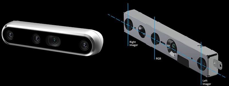
If we observe, for example, a Realsense D455 camera, we will see the two grayscale cameras on the most left and right side of the camera. The middle one is the IR projector and a RGB camera.
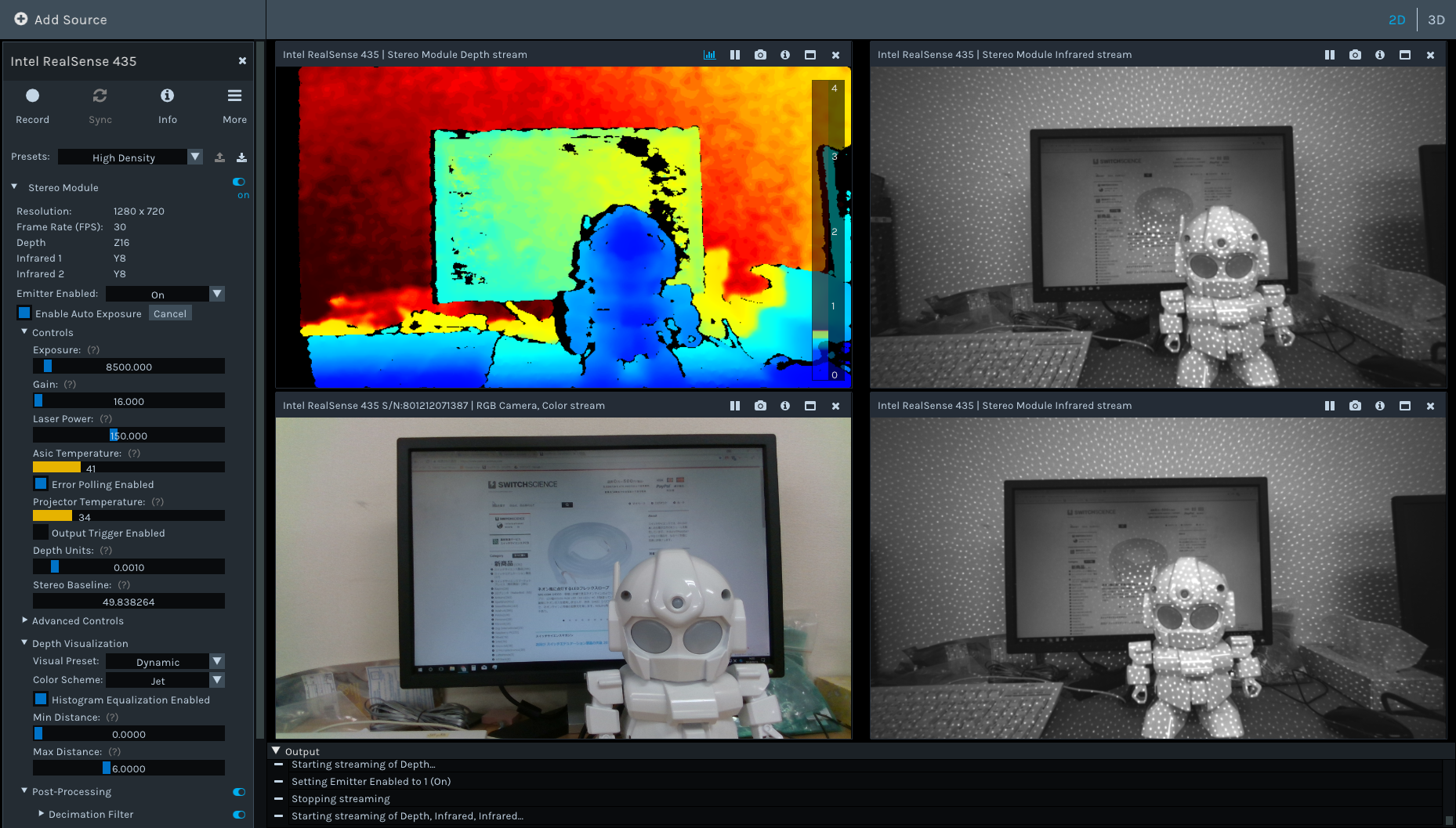
The IR projector is used to project the IR pattern, e.g. dots, into un-textured regions, to improve the robustness of stereo matching for depth computation.
Time-of-Flight (ToF) Cameras
Another type of common camera is the Time-of-Flight (ToF) camera. It provides more accurate depth measurements, but its measurement range is often shorter, usually up to 5 meters. As the name suggests, ToF sensor emits IR light and measures the time it takes for light to travel to objects and back, and then calculate the distance to the objects.
Azure Kinect was a popular ToF camera, but unfortunatly it is now discontinued. However, we still have many good choices for ToF sensors, such as OAK-D TOF, Orbbec Femto Bolt, etc. We can check out these videos to see the depth quality of Orbbec Femto Bolt. here and here.
In fact, LiDAR works in a similar principle as ToF cameras. The difference is that LiDAR uses a laser pulse with higher frequency, and it can reach to much longer distances.
References
- Visual SLAM: From Theory to Practice, by Xiang Gao, Tao Zhang, Qinrui Yan and Yi Liu
- Multiview Geometry in Computer Vision, by Richard Hartley and Andrew Zisserman
If you find this article helpful, please consider citing it in your research:
@article{Hu2026learnvslam,
  author = {Hu, Yafei},
  title = {Learning Visual SLAM: Cameras, Sensors and Projection Model},
  year = {2026}
}